|
SFWMD RSM PEER REVIEW 2019: Draft Report
|
This Draft Report contains Panelist Victor M. Ponce's
contributions and recommendations
after attending the
South Florida Water Management District (SFWMD)
Peer Review of the Regional Simulation Model's (RSM),
held in West Palm Beach, Florida, on July 24-25,
2019.
This review has concluded that the methodologies included in RSM are adequate for its use in south Florida. To improve and complement current efforts, the author recommends that District scientists spend additional time on the issues of numerical accuracy, particularly on the determination of the applicable Courant and cell Reynolds numbers for specific model runs. The author's experience in this area is offered to serve as a suitable framework for the analysis.
1. On strategies for model control to manage instabilities
All numerical models, and RSM is no exception, have a way of becoming unstable under a certain set of circumstances. Thus, it seems appropriate, at the start, to provide a general discussion on strategies for model control to manage instabilities. A good physically based mathematical model is based on generally accepted partial differential equations describing the relevant physical processes. RSM uses 1-D and 2-D formulations of watershed, channel, reservoir, and groundwater flow, coupling them as appropriate to better represent the physical reality at the chosen level of abstraction.
All numerical models suffer from problems of stability and convergence.
Stability is related to roundoff errors; convergence to discretization
errors (O'Brien et al., 1950).
Convergence, which is akin to accuracy (in the sense of convergence to
the analytical solution), is determined by the
size of the discretization, i.e., the values of the discrete
space and time steps, which are chosen by the person performing the modeling.
In practice, the control of numerical instability is seen to be a careful balancing act: How to build a scheme that has enough numerical diffusion to handle the high-frequency perturbations that are responsible for the instability, while at the same time making sure that the solution itself is not being substantially affected by the artificially introduced numerical diffusion. This dilemma is at the crux of all numerical modeling.
The laws of mass and momentum conservation, which underpin all physical-process modeling of unsteady flows, may be combined, through appropriate linearization, into a single second-order, convection-diffusion equation (Hayami, 1951). In one extreme, when the diffusion term vanishes, the equation becomes hyperbolic; in the other extreme, when the convection term vanishes, the equation becomes parabolic.
Numerical models of hyperbolic systems are subject to the
Courant law, which expresses the ratio of physical celerity (c) to numerical celerity
(Δx/Δt), also referred to as the grid ratio. On the other hand, numerical models of parabolic systems
are subject to what has sometimes been referred to (for lack of a better name)
as the cell Reynolds number law,
which expresses the ratio of physical diffusivity (ν) to
numerical, or grid, diffusivity [(Δx)2/Δt].
Both Courant and cell Reynolds numbers control the properties of numerical models
of unsteady flow; their values should be calculated a priori
(Ponce
The properties of numerical schemes may be analyzed using various tools
of advanced mathematics.
In hyperbolic systems, an assessment of numerical accuracy (i.e., convergence) focuses on the spatial resolution L /Δx, where L is the predominant wavelength of the perturbation and Δx is the chosen space step. Generally, numerical models of hyperbolic systems are shown to be more accurate when the grid size follows the characteristic lines, i.e., for a Courant number C = 1, wherein the physical celerity c matches the grid ratio Δx/Δt. In theory, selecting a sufficiently high spatial resolution, say, L /Δx ≥ 100 and a Courant number C = 1 should suffice. In practice, however, a certain scheme may lack enough numerical diffusion to confront the high-frequency perturbations that are likely to appear in well-balanced schemes; thus, additional filtering (numerical diffusion) is normally required to render the system workable.
For instance, there is a wealth of accumulated experience on the numerical properties of the well-known Preissmann scheme, wherein stability and convergence are determined by the spatial resolution L /Δx, the Courant number C, and the weighting factor θ (Ponce et. al., 1978). The latter is required to control nonlinear instabilities which tend to plague the computation as the scheme approaches second order. Values of the weighting factor in the range 0.55 ≤ θ ≤ 1 are recommended, with values near the lower limit approaching convergence (to second order) at the expense of stability, and values near the upper limit approaching stability at the expense of convergence.
An excellent example of the use of Fourier analysis in numerical modeling of flood flows is that of the Muskingum-Cunge model, a diffusion wave model that is based on the matching of physical and numerical diffusivities (Cunge, 1969). A review of the amplitude and phase portraits of the Muskingum-Cunge model, including an online calculator, has recently been accomplished by Vuppalapati and Ponce (2016).
2. On the appropriateness of the TVDLF model implemented in RSM
In its newest implementation, the RSM model uses the Total Variation Diminishing Lax-Friedrichs method (TVDLF), which is shown to be accurate and stable for both kinematic and diffusion flows such as those prevalent in Southern Florida (Lal and Gabor, 2013). The method uses a linearized conservative implicit formulation of the simplified St. Venant equations, thereby avoiding the iterative formulations that would normally be necessary when solving a nonlinear scheme. SFWMD scientists have extensively tested the method, with favorable results in terms of numerical accuracy and runtime.
The success of the method in simulating a wide array of problems, including dry channel bed and steep bottom slopes, must be attributed to its use of weighting factors to incorporate numerical diffusion as needed to control the instabilities that would normally appear in connection with sharp (i.e., nonlinear) changes in model variables. The author welcomes the use of the TVDLF method and supports its continued use; the downside, however, is the increased level of complexity, compared to more conventional methods.
3. On the use of a dynamic hydraulic diffusivity in convection-diffusion modeling of surface runoff
An established approach to modeling flood flows used in RSM
is that of Hayami (1951), who combined the governing
equations of continuity and motion (the Saint Venant equations)
into a second-order partial
differential equation with discharge Q as the dependent variable.
This equation, effectively a convection-diffusion model of surface runoff,
has been widely used in practice. It consists of: (1) a rate-of-rise term,
(2) a convective term, of first order, and (3)
a diffusive term, of second order.
The hydraulic diffusivity used in RSM follows the original Hayami formulation
of a diffusion wave, wherein the inertia terms (in the equation of motion)
are neglected. This approximation works well for low Froude number flows.
However, for high Froude number flows, the neglect of inertia proves to be increasingly
unjustified. As shown in Ponce (1991), the true hydraulic diffusivity
of the convection-diffusion model of flood flows
is the dynamic hydraulic diffusivity, which
is a function of the Vedernikov number
We recommend that a dynamic hydraulic diffusivity be incorporated into all instances where surface-water convection-diffusion is being modeled in RSM. This extension provides a lot of bang for the buck, since the structure of the computation remains basically the same. Ponce's formulation clarifies the work of Dooge and his associates, as recounted recently by Nuccitelli and Ponce (2014).
4. On the choice of spatial resolution for good modeling practice
The determination of the proper spatial resolution
lies at the crux of good modeling practice, as the experience with RSM clearly shows.
No amount of time spent on this effort is wasted.
Our recommendation is to start with a
target spatial resolution
|
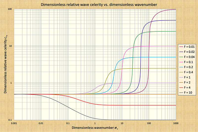
Fig. 1 Dimensionless relative wave celerity vs dimensionless wavenumber in open-channel flow.
5. On the comparative advantages of implicit vs explicit schemes
The choice between explicit and implicit schemes continues to haunt numerical modelers. While implicit schemes are unconditionally stable, a similar statement may not follow for explicit schemes. This is certainly the case for both surface and groundwater flows. On this basis, implicit schemes are generally preferred over explicit schemes, but the complete story remains to be told.
It may be true that implicit schemes are not subject to an upper limit on the time step
in order to remain stable.
However, the use of time steps greatly exceeding this limit renders
the model inaccurate
(nonconvergent). Thus, the use of implicit schemes with Courant numbers greatly exceeding 1 (C >> 1) must be
viewed with extreme caution, begging for a Fourier analysis for proof of convergence.
Furthermore, certain explicit schemes are not
subject to a stability condition, as demonstrated by
Ponce
The tradeoffs between explicit and implicit schemes are, therefore, clear:
While implicit schemes are more stable,
they require matrix inversion and the actual
time step is effectively limited in size by accuracy considerations.
Explicit schemes, on the other hand, are simpler to develop and execute,
requiring no matrix inversion and no downstream boundary
(Ponce
6. On the need to use the full unsteady flow equations for flow in a horizontal channel
In the typical case, the forces acting on a 1-D formulation of
unsteady open-channel flow are: (1) gravity,
(2) friction, (3) pressure gradient, and (4) inertia.
Significantly, in a horizontal channel the gravitational force vanishes,
while the three other forces remain.
This renders the Manning equation inapproriate, since the driving force
in this equation is the gravitational force. Thus,
for modeling unsteady flows in
horizontal channels (the case of south Florida) there appears to be no other choice
than to use
the full Saint-Venant equations.
The need to include lateral contributions (seepage in and out of the control volume) in the analysis of wave propagation in south Florida applications remains to be fully clarified. Great strides along these lines have already been made by SFWMD scientists. The additional terms in the mass and momentum balance equations need to be carefully identified. Their relative importance may be determined following the work of Ponce (1982).
7. On the need for RSM model version numbers
The term "RSM model" is being currently used to describe any and all
activities under the RSM modeling framework. This explains
the District's (SFWMD) reluctance
to engage in explicit model version numbers to describe what amounts to
activities of varied scope and in many areas.
8. On the need for consistency in model documentation
We recommend that SFWMD consider a thorough and full documentation of the RSM model via a technically edited User Manual, accompanied by a Reference Manual, as a way to ensure that potential users of the model will be able to use it in the future. Background material would consist of relevant published papers listed in the bibliography and included therein with hot links to online pdf files.
As an alternative, one certainly requiring fewer resources, the District could sponsor a publications series to be entitled, for example, RSM Tecnical Monographs. For consistency, each monograph would follow the same (or similar) format and describe in detail a specific portion of the model, using graphics and color as appropriate. This approach has the advantage that progress is not defined in terms of project completion.
9. Other miscellaneous recommendations
We offer the following miscellaneous recommendations:
The 2-D momentum equations originate in the 3-D Navier-Stokes equations, and, as such, are technically not closed (Flokstra, 1976; 1977). Some sort of surrogate for the missing effective stresses appears in order (Kuipers and Vreugdenhil, 1973). This is an obscure subject, perhaps deserving of more attention than that given so far.
Caution is recommended when using a 2-D formulation of a diffusion wave, wherein the inertia terms are neglected. Neglecting inertia is bound to eliminate physical circulation (Ponce and Yabusaki, 1981). However, it may be a reasonable assumption in the largely convective 2-D flows that prevail in south Florida.
The Muskingum-Cunge model of 1-D flood flows, effectively a diffusion wave model, has been analytically verified by Ponce et al. (1996). We suggest that the District consider including this verification test in their set of cases for model verification.
References
Cunge, J. A.. 1969.
On the subject of a flood propagation computation method (Muskingum method). Journal of Hydraulic Research, Vol. 7, No. 2, 205-230.
Flokstra, C. 1976. Generation of two-dimensional horizontal secondary currents.
Report S 163-II, Delft Hydraulics Laboratory, Delft, The Netherlands, July.
Flokstra, C. 1977. The closure problem for depth-averaged two-dimensional
flow.
Paper A106,
17th Congress of the International Association for Hydraulic Research,
Baden-Baden, Germany, Vol. 2, 247-256.
Hayami, S. 1951. On the propagation of flood waves. Bull.
Disaster Prev. Res. Inst. Kyoto Univ., 1, 1-16.
Kuipers, J. and C. B. Vreugdenhil. 1973. Calculations of two-dimensional
horizontal flows. Report S 163-I, Delft Hydraulics Laboratory, Delft, The Netherlands, Oct.
Lal, A. M. and G. Toth. 2013. Implicit TVDLF methods for diffusion and kinematic flows. Journal of Hydraulic Engineering, ASCE,
Vol. 139, No. 9, September, 974-983.
Leendertse, J. J. 1967. Aspects of a computational
model for long-period water wave propagation.
RM-5294-PR, The Rand Corporation, Santa Monica, Calif., May.
Lighthill, M. J. and Whitham, G. B. 1955. On
Kinematic Waves I, Flood Movement in Long Rivers.
Proceedings of the Royal Society of London, Vol. A229, May, 281-316.
Nuccitelli, N. R. and V. M. Ponce. 2014.
The
dynamic hydraulic diffusivity reexamined.
O'Brien, G. G., M. A. Hyman and S. Kaplan. 1950.
A
study of the numerical solution of partial differential equations.
Journal of Mathematics and Physics, Vol. 29, No. 4, 231-251.
Ponce, V. M. and D. B. Simons. 1977. Shallow
wave propagation in open-channel flow.
Journal of the Hydraulics Division, ASCE, Vol. 103, HY12, Proc. Paper, 13392. Dec., 1461-1476.
Ponce, V. M., H. Indlekofer and D. B. Simons. 1978. Convergence
of four-point implicit water wave models.
Journal of the Hydraulics Division, ASCE, Vol. 104, HY7,
July, 947-958.
Ponce, V. M. and S. B. Yabusaki. 1981.
Modeling
circulation in depth-averaged flow.
Journal of the Hydraulics Division, ASCE, Vol. 101, HY11,
November, 1501-1518.
Ponce, V. M. 1982.
Nature of wave attenuation in open-channel flow.
Journal of the Hydraulics Division, ASCE, Vol. 108, HY2,
February, 257-262..
Ponce, V. M. 1991. New
perspective on the Vedernikov number. Water Resources Research, 27(7), 1777-1779.
Ponce, V. M., A. K. Lohani and C. Scheyhing. 1996.
Analytical verification of Muskingum-Cunge
routing. Journal of Hydrology, Vol. 174, 235-241.
Ponce, V. M., A. V. Shetty and S. Ercan. 2001.
A
convergent explicit groundwater model.
Ponce, V. M. 2014.
Fundamentals of open-channel hydraulics. An online textbook.
Powell, R. W. 1948.
Vedernikov's criterion for ultra-rapid flow.
Transactions, American Geophysical Union,
Vol. 29, No. 6, 882-886.
Vuppalapati, B. and V. M. Ponce. 2016. Muskingum-Cunge
amplitude and phase portraits
with online computation. An online pubs+calc publication.