1.  INTRODUCTION

A stable-and-convergent numerical groundwater model is developed herein. Stability being a necessary condition for model operation, the emphasis is on convergence, i.e., whether the numerical model can reproduce the differential equation with sufficient accuracy.

A significant feature of the model is its simplicity, which makes it attractive and useful for a wide variety of applications. The numerical model is an explicit formulation of the two-dimensional (x-y) diffusion equation of flow in porous media for a homogeneous isotropic aquifer. Sources (percolation from rainfall and/or irrigation) and sinks (pumping) are accounted for in the formulation. Boundary conditions are specified as: (a) head or flux, and (b) permeable or impermeable.

A specific focus of the model development is the assessment of stability and convergence. Explicit models are subject to a strict stability criterion, which must be satisfied if the model is to simulate natural conditions in a realistic way (O'Brien et al. 1949; Douglas 1956). As shown herein, the model must also satisfy a convergence criterion if accuracy is to be maintained. The satisfaction of both stability and convergence requires that the cell Reynolds number D be equal to 1.

After more than 20 years of implicit model development of groundwater flow, the choice of an explicit model at this juncture requires further explanation. It is well known that implicit models are unconditionally stable. Lesser known is the fact that implicit models are subject to a convergence criterion which effectively places an upper limit on the time step. Examples of lack of convergence in surface-water and sediment-transport modeling have been documented by Ponce et al. (1978; 1979). Thus, when their additional complexity is factored in, implicit models may not be necessarily better than explicit models.

2.  MODEL FORMULATION

The three-dimensional diffusion equation for flow through porous media is (Rushton and Redshaw 1979; Kresic 1997):

∂               ∂h             ∂             ∂h             ∂              ∂h                           ∂h ____ ( Kx  _____ )  +  ____ ( Ky _____)  +  ____ ( Kz _____ )  +  W  =  Ss  ____  ∂x              ∂x            ∂y            ∂y             ∂z             ∂z                           ∂t

(1)

in which h = piezometric head [ L ]; K_x, K_y, and K_z are the hydraulic conductivities along the x , y , and z coordinate axes, respectively [ L T ^-1]; W = volumetric flux per unit volume, representing sources (+) or sinks (-) [ T ^-1]; S_s = specific storage of the porous material [ L^-1]; and t = time.

In two dimensions in plan, Eq. 1 simplifies to:

∂               ∂h             ∂             ∂h                           ∂h ____ ( Kx  _____ )  +  ____ ( Ky _____)  +  W  =  Ss  ____  ∂x              ∂x            ∂y            ∂y                            ∂t

(2)

Assuming a homogeneous isotropic aquifer of hydraulic conductivity K:

∂2h        ∂2h                           ∂h  K (  _____  +  _____ ) +  W  =  Ss  ____           ∂x2         ∂y2                          ∂t

(3)

Defining the hydraulic diffusivity of the aquifer (Freeze and Cherry 1979) as follows:

K  ν =  _____            Ss

(4)

leads to:

∂2h        ∂2h          νW          ∂h  ν ( _____  +  _____ ) +  _____  =  ____          ∂x2        ∂y2            K           ∂t

(5)

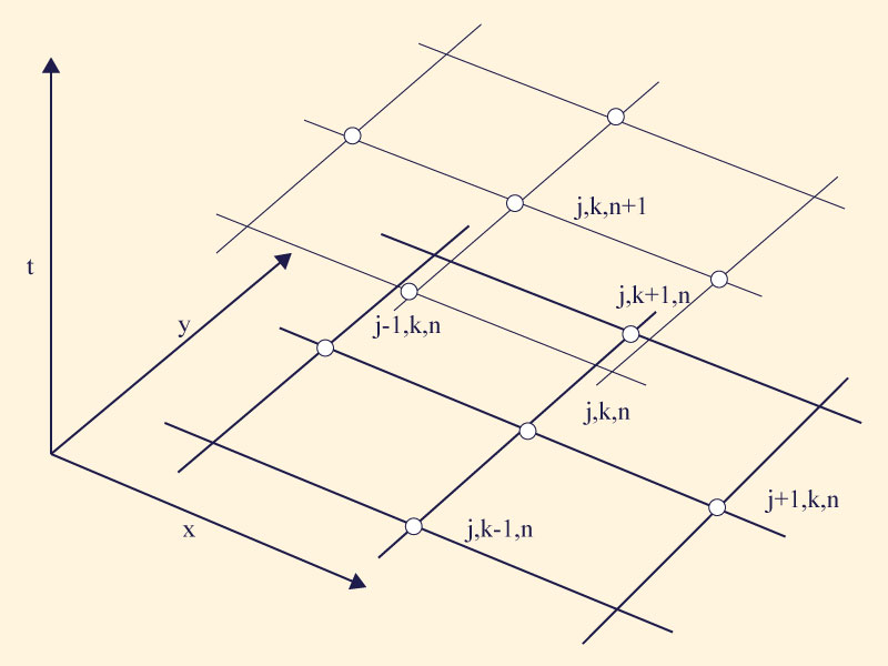
Equation 5 represents two-dimensional flow in a homogeneous isotropic aquifer of properties K and ν, and source/sink term W. A simple and appropriate finite-difference scheme of first order in time and second order in space is (Fig. 1):

n + 1      n                n           n        n                 n           n        n     hj,k    - hj,k             hj+1,k - 2hj,k  + hj-1,k           hj,k+1  - 2hj,k + hj,k-1         ν ___________ =   ν  ___________________ +  ν __________________ + ( ____ ) Wj,k        Δt                              (Δx)2                                (Δy)2                 K

(6)

Fig. 1   Notation for finite-difference scheme.

The spatial interval is set as Δs = Δx = Δy. Following Roache (1972), we define a type of cell Reynolds number as the ratio of physical and numerical diffusivities. This leads to:

ν                   Δt D  =  ________  =  4ν  ______           (Δs /2)2            (Δs)2           _______               Δt

(7)

Eq. 6 reduces to:

n+1           n                        n              νΔt h j, k  =  D h̄ j, k +  ( 1 - D ) h j, k   +  ( _____ ) Wj, k                                                              K

(8)

In which:

n               n               n               n                 h j +1, k  +  h j -1, k  +  h j, k+1  +  h j, k -1                                                     n h̄ j, k =     _____________________________________________                                             4

(9)

The time-averaged source term, in velocity units, is the following:

r j, k W j, k =   ______                   b

(10)

in which r_j,k = percolation rate [L T^-1] (due to rainfall and/or irrigation) at spatial node (j, k), and b = aquifer depth [L].

The time-averaged sink term, in discharge units, is the following:

p j, k W j, k =  -  ________                  b (Δs)2

(11)

in which p_j,k = pumping rate [L³ T^-1] at the spatial node (j,k).

Since transmissivity is:

T = Kb

(12)

and diffusivity is:

T ν =  _____          S

(13)

in which S = storage coefficient (Freeze and Cherry 1979), Eq. 8 reduces to the following:

n+1            n                       n               Δt                          Δt h j, k  =  D h̄ j, k +  ( 1 - D ) h j, k   +  ( _____ ) r j, k  -  [ _________ ] p j, k                                                              S                      S (Δs)2

(14)

With Eqs. 7 and 13, Eq. 14 reduces to the following:

n+1            n                         n             D (Δs)2                    D h j, k  =  D h̄ j, k  +  ( 1 - D ) h j, k   +  [ ________ ] r j, k  -  ( _____ ) p j, k                                                                4T                        4T

(15)

For the special case D = 1, Eq. 15 reduces to:

n+1         n            (Δs)2                    1 h j, k  =  h̄ j, k  +  [ ______ ] r j, k  -  ( _____ ) p j, k                               4T                      4T

(16)

Equation 15 calculates piezometric head at the unknown node (j, k, n+1) based on the average piezometric head h̄ _{j, k} ⁿ at the four known nodes adjacent to (j, k, n), the percolation rate r_j,k, the pumping rate p_j,k, the space interval Δs, and the transmissivity T (Fig. 1).

3.  BOUNDARY CONDITIONS

The boundary conditions can be of Dirichlet or Neumann type (Kinzelbach 1986). Dirichlet conditions specify the head h; Neumann conditions specify the flux, i.e., the head gradient ∂h/∂x orthogonal to the boundary. In general, Dirichlet conditions lead to a permeable boundary, since the flux is usually finite. Neumann conditions are type A (permeable) or type B (impermeable). A Neumann type A condition specifies a finite gradient, i.e., ∂h/∂x ≠ 0; on the other hand, a Neumann type B condition specifies a zero gradient, i.e., ∂h/∂x = 0.

Neumann type A boundaries may be specified by linear extrapolation from the two immediately neighboring interior nodes. Linear extrapolation results in a finite gradient, which amounts to a permeable boundary. Neumann type B boundaries may be specified by relocation of the neighboring interior node; relocation results in a zero gradient, which amounts to an impermeable boundary.

Mixed Neumann type A/type B conditions, appropriate for semipermeable boundaries or temporally varying inflows, may be specified as follows:

n+1                       n+1               n+1 h j, k  =  ( 1 + α ) h j - 1 ,k  -  αh j - 2 ,k

(17)

in which j = boundary node, and α = weighting factor, varying in the range 0 ≤ α ≤ 1, such that α = 0 represents an impermeable boundary, and α = 1 a permeable boundary.

4.  MODEL TESTING

The model was subjected to the following four tests to examine its numerical properties:

1. Permebale hot-start test

This condition tests the model's ability to return to the steady-equilibrium baseline condition following the specification of: (a) a depleted water table as initial condition, (b) permeable boundaries, and (c) no pumping.

2. Permeable cold-start test

This condition tests the model's ability to achieve a steady-equilibrium cone of depression following the specification of: (a) the baseline steady-equilibrium initial condition, (b) permeable boundaries, and (c) pumping.

3. Impermeable hot-start test

This condition tests the model's ability to return to a steady-equilibrium nonbaseline condition following the specification of: (a) a depleted water table as initial condition, (b) impermeable boundaries, and (c) no pumping.

4. Impermeable cold-start test

This condition tests the model's ability to simulate the linear depletion of the aquifer following the specification of: (a) the baseline steady-equilibrium initial condition, (b) impermeable boundaries, and (c) pumping.

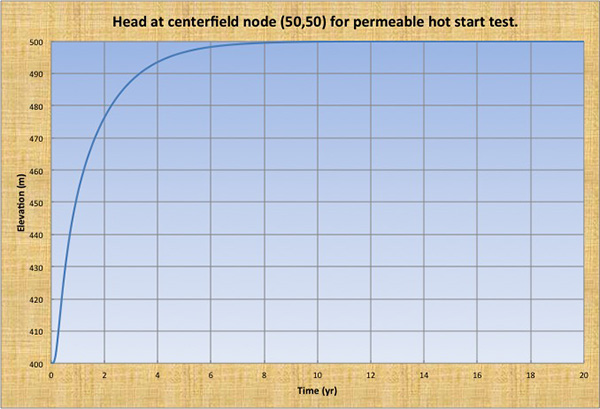
Convergence testing

First, the groundwater model was tested for convergence (O'Brien et al. 1949). For this purpose, a permeable hot-start test was used, wherein the (complete, i.e., full) head recovery to steady-equilibrium baseline condition is a proof of the model's convergence.

The test prototype specification was a 100-km² square aquifer (10 km x 10 km) of transmissivity T = 0.01 m² s^-1 and storage coeficient S = 0.1. Given Eq. 13, the hydraulic diffusivity is ν = 0.1 m² s^-1. The space interval was set as Δs = 100 m, i.e., a total of 101 × 101 = 10201 grid nodes, labeled (0,0) to (100,100).

Stability requires that D ≤ 1. Therefore, D = 1 is the maximum cell Reynolds number that can be used in practice. For D = 1, the time interval is fixed at the following value (Eq. 7):

(Δs)2 Δt  =  ______              4ν

(18)

A series of sixteen (16) runs were performed to test the convergence of the groundwater model under varying cell Reynolds number D and reference head h_ref (steady-equilibrium baseline condition). The initial condition was specified as h₀ = (h_ref - 100) in a square area of 5 km × 5 km located in the middle of the computational field (51 × 51 = 2601 grid nodes).

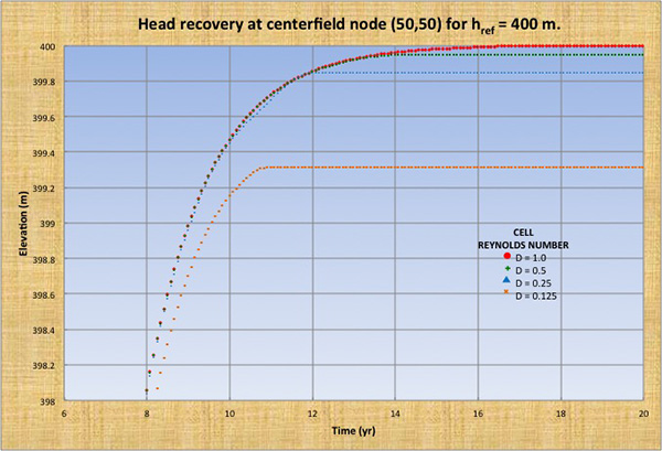
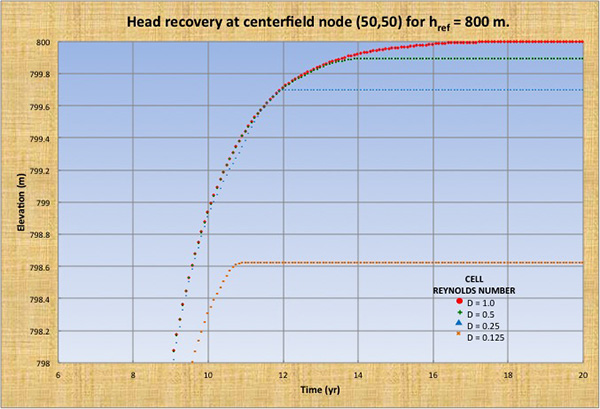
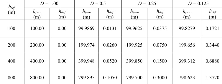
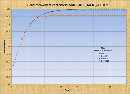
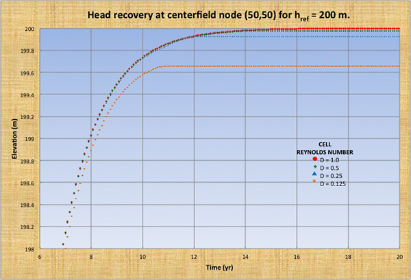
Four cell Reynolds numbers (D = 1.0, 0.5, 0.25, and 0.125) and four reference heads (h_ref = 100, 200, 400 and 800 m) were chosen for the test series. The aquifer bottom was set at h_bottom = 0 m. From Eq. 18, the time interval for D = 1.0 is Δt = 6.944 hr. Therefore, the time intervals to be used in the test series are: Δt = 6.944, 3.472, 1.736, and 0.868 hr, corresponding to D = 1.0, 0.5, 0.25, and 0.125, respectively.

Figures 2 (a) to (d) show head recovery at centerfield node (50, 50) for reference heads h_ref = 100, 200, 400, and 800 m, and cell Reynolds numbers D = 1.0, 0.5, 0.25, and 0.125. For values other than D = 1, a head recovery deficit is present, signaling the model's inability to return to steady-equilibrium baseline condition, i.e., lack of convergence. Table 1 shows the head recovery deficit h_def as a function of reference head h_ref and cell Reynolds number D.

Table 1. Head recovery deficit hdef as a function of reference head href and cell Reynolds number D.

Fig. 2 (a)  Head recovery at centerfield node (50,50) for href = 100 m.

Fig. 2 (b)  Head recovery at centerfield node (50,50) for href = 200 m.

Fig. 2 (c)  Head recovery at centerfield node (50,50) for href = 400 m.

Fig. 2 (d)  Head recovery at centerfield node (50,50) for href = 800 m.

The following conclusions are drawn from Fig. 2 and Table 1:

1. The head recovery deficit h_def = 0, i.e., the head recovery is complete, only for D = 1.

2. The head recovery deficit increases nonlinearly with decreases in cell Reynolds number from 1.0 to 0.125.

3. The head recovery deficit increases linearly with increases in reference head from 100 to 800 m.

4. The condition D = 1 is not only the most accurate but also the most economical. For smaller values of D, the model is less convergent and the run takes more processor and total time to complete.

Permeable/impermeable hot/cold tests

The permeable/impermeable hot/cold tests were carried out by specifying the same geometry and aquifer properties as for the convergence test runs. The cell Reynolds number was set at D = 1, which leads to Δt = 6.944 hr.

For the hot tests, the reference head is set at h_ref = 500 m and the initial condition is specified as h₀ = (h_ref - 100) in a square area of 5 km × 5 km located in the middle of the computational field. The aquifer bottom is set at h_bottom = 0 m. Thus, the steady-equilibrium aquifer volume is 50,000 hm³.

For the cold tests, the reference head href = 500 m is specified as initial condition at every node and the aquifer bottom is set at h_bottom = 0 m. Thus, the steady-equilibrium aquifer volume is 50,000 hm³. A battery of seventeen (17) pumps is symmetrically positioned across the field, at a distance of 1,414.2 m apart, making the shape of an X (Fig. 3), and each pumping p = 250 L s^-1.

Fig. 3  Pump locations for cold start tests.

Permeable hot-start test

The initial aquifer volume is 47,399 hm³. The piezometric level returned to steady-equilibrium condition (h = 500 m at every node) in an asymptotic fashion after 15.85 yr of simulation (Fig. 4). The simulation was strongly stable and convergent. The calculated aquifer volume, after attainment of the steady-equilibrium condition, was 50,000 hm³.

Fig. 4  Head at centerfield node (50,50) for permeable hot start test.

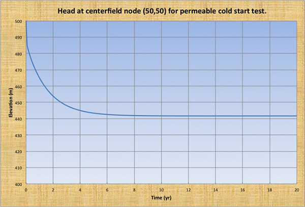
Permeable cold-start test

The initial aquifer volume is 50,000 hm³. The piezometric level reached a steady-equilibrium condition, with the maximum depletion (h = 441.662 m) at the centerfield node (50,50), in an asymptotic fashion after 12.43 yr of simulation (Fig. 5). The simulation was strongly stable. The calculated aquifer volume was 48,218 hm³. The volume conservation, calculated by taking the initial aquifer volume, subtracting the pumped volume and adding the boundary inflows, was 99.98 percent at the end of the 20-yr simulation.

Fig. 5  Head at centerfield node (50,50) for permeable cold start test.

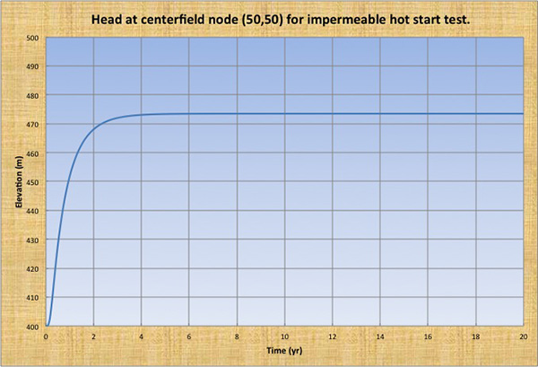
Impermeable hot-start test

The initial aquifer volume is 47,399 hm³. The piezometric level reached a steady-equilibrium condition (h = 473.462 m at every node) in an asymptotic fashion after 8.34 yr of simulation (Fig. 6). The simulation was strongly stable. The calculated aquifer volume, after achievement of the steady-equilibrium condition, was 47,349 hm³. The volume conservation, calculated as the ratio of calculated to initial aquifer volume, was 99.89 percent at the end of the 20-yr simulation.

\ Fig. 6  Head at centerfield node (50,50) for impermeable hot start test.

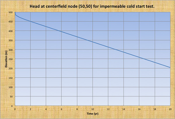
Impermeable cold-start test

The initial aquifer volume is 50,000 hm³. The piezometric level decreased in a linear fashion, with the maximum depletion (h = 203.905 m) at the centerfield node (50,50) after 20 yr of simulation (Fig. 7). The simulation was strongly stable. The calculated aquifer volume at the end of the 20-yr simulation was 22,687 hm³, i.e., 45.37% of the initial aquifer volume.

Fig. 7  Head at centerfield node (50,50) for impermeable cold start test.

5.  SUMMARY AND CONCLUSIONS

A stable-and-convergent two-dimensional groundwater model of a homogeneous isotropic aquifer has been developed and tested under a wide range of flow conditions. The model is explicit and can account for the following: (a) sources/sinks, and (b) head/flux or permeable/impermeable boundaries. A significant feature of the model is that it sets the cell Reynolds number D = 1 to satisfy both stability and convergence.

Testing of the model under hypothetical conditions showed that the model is stable, convergent, and mass conservative. The permeable hot-start test converged to the steady-equilibrium baseline condition after 15.85 yr. The permeable cold-start test converged to a steady-equilibrium cone of depression after 12.43 yr. The impermeable hot-start test converged to a steady-equilibrium non-baseline condition after 8.34 yr. The impermeable cold-start test properly simulated the linear depletion of the aquifer.

References

Douglas, Jr., G. 1956. On the relation between stability and convergence in the numerical solution of linear parabolic and hyperbolic equations. Journal of Society of Industrial and Applied Mathematics, 4, 20-37.

Freeze, and Cherry. 1979. Groundwater. Prentice Hall, Englewood Cliffs, New Jersey.

Kilzenbach, W. 1986. Groundwater modelling: An introduction with sample programs in BASIC. Developments in Water Science No. 25, Elsevier, Amsterdam, The Netherlands.

Kresic, N. 1979. Quantitative solutions in hydrogeology and groundwater modeling. Lewis Publishers, New York.

O'Brien, G. G. Hyman, and M. A. Kaplan. 1950. A study of the numerical solution of partial differential equations. Journal of Mathematics and Physics, 29(4), 231-251.

Ponce, V. M., H. Indlekofer, and D. B. Simons. 1978. Convergence of four-point implicit water wave models. Journal of the Hydraulics Division , ASCE, 104(HY7), 947-958.

Ponce, V. M., H. Indlekofer, and D. B. Simons. 1979. The convergence of implicit bed transient models. Journal of the Hydraulics Division, ASCE, 105(HY4), 351-363.

Roache, P. 1972. Computational fluid dynamics. Hermosa Publishers, Albuquerque, NM.

Rushton, K. R., and S. C. Redshaw. 1979. Seepage and groundwater flow; numerical analysis by analog and digital methods. John Wiley and Sons, New York.