USING ONLINE COMPUTATION
Janaina A. Da Silva
ACKNOWLEDGEMENTS
This thesis is dedicated to Dr. Victor Miguel Ponce, whose life's work made possible the completion
of this project. Everyone who knows him knows his commitment to greatness and the passion with which
he teaches and expresses himself through his work. The time spent producing this thesis was a time
full of lessons, not only about engineering but also about human behavior and relationships.
The decisions we make forge our character. The process through fire is uncomfortable and painful,
but it transforms us into exactly what we need to be to face the next phase in our lives. It teaches
and prepares us, and for that, I'm grateful.
My gratitude also goes to thesis Committe members Dr. Hassan Tavakol-Davani and Dr.
Subrata Bhattacharjee for their support as part of my thesis committee.
Thank you for taking an interest in our work.
1. INTRODUCTION
1.1 Background As the world's population continues to grow, and consequently the demand for water, better water management has become more important. In the past eight decades, with the advent of rural electrification and more effective drilling and pumping technologies, groundwater began to be extensively used as a source of water supply (Reilly et al., 2008). With the increase in groundwater utilization came the need for a better understanding of not only its behavior but also its relation with surface water and vegetation, as well as its role in contaminant dispersion. A meaningful assessment of groundwater requires a multidisciplinary evaluation of the hydrologic system, as well as an understanding of the different water issues that exist across the world (Reilly et al., 2008). Groundwater modeling is an important tool in this assessment, given the dramatic increase in its role on water management since the 1980s (Refsgaard et al., 2010). One of the objectives of a numerical groundwater model is to predict the aquifer's behavior under different scenarios of groundwater utilization. It is important to note that all models are simplifications of reality; therefore, they will not be precisely accurate. This fact was well stated by the National Research Council (2007) as follows:
Advances in groundwater modeling have been accomplished not only in the fields of hydrogeology and groundwater hydrology, but also in related fields, such as computational fluid dynamics, petroleum reservoir modeling, climatological modeling, and geophysics (Langevin and Panday, 2012). Groundwater models may grow in complexity depending on the intended use. In this thesis, we focus on a convergent explicit groundwater model to analyze unconfined alluvial aquifer depletion and recovery. An assessment of the available groundwater models reveals a wide range of software packages, varying from a comprehensive numerical model available in the public domain (MODFLOW) to relatively advanced three-dimensional graphical models, which are usually proprietary. Two common factors may be observed in the available software packages:
The online groundwater model presented here overcomes these obstacles. The interface is designed to be highly intuitive and the model may be accessed from any computer connected to the internet. 1.2 Objectives The overall objective is to develop a convergent explicit groundwater model suited to online computation. For this purpose, we follow Ponce et. al.'s pioneering work on convergent explicit groundwater modeling (Ponce et al., 2001). They used an explicit formulation of the two-dimensional diffusion equation of flow in porous media, applicable to a homogeneous isotropic aquifer, to obtain a stable and convergent numerical groundwater model. A significant feature of the model is its unusual simplicity, which makes it attractive and useful for a wide variety of applications, including its use as a teaching and learning tool. Ponce et. al. (2001) explains the choice for an explicit groundwater modeling as follows:
A 100-km2 aquifer, of square shape, with transmissivity T and specific yield S, is used to demonstrate the operation, testing, and application of the model. Four scenarios are considered.
Table 1.1 shows the testing scenarios considered.
In this thesis, an online convergent explicit groundwater model ONLINEGWMODEL.PHP is developed by converting the FORTRAN77 code of Ponce et al. (2001) into the PHP language. The input/output interface is accomplished using HTML. PHP is an open-source, server-side scripting language, i.e., the data is processed in the server before the output is delivered to the user. PHP is in the public domain, runs in practically all platforms, is compatible with almost all servers, and supports a wide variety of databases.
Rasmus Lerdorf created PHP in 1994 using a
set of Common Gateway Interface (CGI) binaries written in the C
programming language. His original purpose
was to track visits to his online resume.
In 1995 Lerdof released the code source to the public,
which allowed developers to use it and improve it.
Many versions of the code followed as PHP gained in popularity
around the world.
HTML is a markup language that defines the structure of the web content. When working together, PHP generates HTML and HTML passes back information to PHP. 1.4 Limitations The groundwater model developed here is a numerical model of deterministic equations. It is based on a finite-difference formulation of the governing partial differential equations of flow through porous media. Therefore, it is not suited for use with stochastic inputs. In addition, the model is a simplified representation of a thoroughly complex system, best suited for online teaching and learning of groundwater flow; as such, it is not suited for use with complex practical situations.
2. THEORETICAL BACKGROUND
2.1 Implicit and Explicit Models The numerical model is an explicit formulation of the two-dimensional (x-y) diffusion equation of flow in porous media, applicable to a homogeneous isotropic aquifer. Explicit models are subject to a stability criterion in order to remain stable (O'Brien et al., 1949; Douglas, 1956). As shown here, the model must also satisfy a convergence criterion if numerical accuracy is to be preserved. The satisfaction of stability and convergence requires that the cell Reynolds number D = 1. After more than 30 years of implicit model development of groundwater flow, the choice of an explicit model at this juncture requires further explanation. It is well known that implicit models are unconditionally stable. Lesser known is the fact that implicit models are subject to a convergence criterion which effectively places an upper limit on the time step. Examples of lack of convergence in surface-water and sediment-transport modeling have been documented elsewhere (Ponce et al. 1978; 1979). Thus, when their additional complexity is factored in, implicit models may not be necessarily better than explicit models. 2.2 Numerical Stability Differential equations may be used to numerically represent complex physical problems. However, the numerical approximations to the differential equations may exhibit unstable behavior. A scheme is said to be stable if a small perturbation in the initial values produces a correspondingly small perturbation in the solution of the difference equation; otherwise, the model is unstable (Gary, 1969). The model's instability is associated with the chosen time and space resolution. Stability is assured by following numerical criteria, which characterize every model. In the field of fluid mechanics, the concept of grid Peclet number is used to relate numerical and physical diffusivities as follows:
In which U = advective velocity [L T-1]; Δx = mesh size; and κ = thermal diffusivity. Roache (1972) replaced the thermal diffusivity κ for the hydraulic diffusivity ν to define the cell Reynolds number:
Ponce (1978) adapted Roache's concept of cell Reynolds number to simplify the Muskingum-Cunge method of flood routing (Chow, 1959; Cunge, 1969). However, Ponce defined the cell Reynolds number as the reciprocal of Roache's, that is, the ratio of physical to numerical diffusivities:
Ponce et al. (2001) extended the cell Reynolds number to the field of groundwater modeling, using the same concept of the ratio of physical and numerical diffusiviies, as follows:
in which ν = aquifer diffusivity. The groundwater model developed herein uses the cell Reynolds number defined by Eq. 2.4 to assure both stability and convergence. The adaptation of the concept of cell Reynolds number to groundwater modeling, pioneered by Ponce et al. (2001), has been documented by Ravazzani et al. (2011). They developed a groundwater model representing two-dimensional flow in unconfined aquifers based on macroscopic cellular automata. Their model represents dynamical systems which are discrete in space and time, operate on a uniform regular lattice, and are characterized by local interaction. 2.3 Numerical Convergence Stability being a necessary condition for model operation, the emphasis shifts to convergence, i.e., whether the numerical model can reproduce the differential equation with sufficient accuracy (O'Brien et al. 1950). Convergence testing is described in detail in Section 4.3. 2.4 Groundwater Modeling The three-dimensional diffusion equation for flow through porous media is (Rushton and Redshaw 1979; Kresic 1997):
in which h = piezometric head [ L ]; Kx, Ky, and Kz are the hydraulic conductivities along the x , y , and z coordinate axes, respectively [ L T -1 ]; W = volumetric flux per unit volume, representing sources (+) or sinks (-) In two dimensions in plan, Eq. 2.5 simplifies to:
Assuming a homogeneous isotropic aquifer of hydraulic conductivity K:
Defining the hydraulic diffusivity of the aquifer (Freeze and Cherry, 1979) as follows:
leads to:
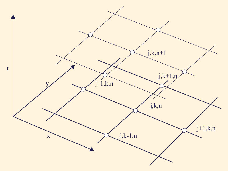
Equation 2.9 represents two-dimensional flow in a homogeneous isotropic aquifer of properties K and ν and source/sink term W. A simple and appropriate finite-difference scheme of first order in time and second order in space is (Figure 2.1):
Figure 2.1 Definition sketch for finite-difference scheme.
The spatial interval is set as Δs = Δx = Δy. Following Ponce et al. (2001), the cell Reynolds number is defined as the ratio of physical and numerical diffusivities, as follows:
Equation 2.10 reduces to:
In which
The time-averaged source term as a function of percolation rate is:
in which rj,k = percolation rate [ L T-1 ] (due to rainfall and/or irrigation) at spatial node (j, k),
and The time-averaged sink term as a function of pumping rate is:
in which pj,k = pumping rate [ L3 T-1 ] at spatial node (j,k). Since transmissivity
and diffusivity
in which S = specific yield (Freeze and Cherry, 1979), Eq. 2.12 reduces to
With Eqs. 2.11 and 2.17, Eq. 2.18 reduces to:
For the special case of D = 1, Eq. 2.19 reduces to:
Equation 2.19 calculates the piezometric head at the unknown node (j, k, n+1) based on the average piezometric head h̄ j, k n at the four known nodes adjacent to (j, k, n), the percolation rate rj,k,
the pumping rate 2.5 Boundary Conditions The boundary conditions can be of Dirichlet or Neumann type (Kinzelbach, 1986). Dirichlet conditions specify the head h; Neumann conditions specify the flux, i.e., the head gradient ∂h/∂x orthogonal to the boundary. In general, Dirichlet conditions lead to a permeable boundary, since the flux is usually finite. Neumann conditions are type A (permeable) or type B (impermeable). A Neumann type A condition specifies a finite gradient, i.e., ∂h/∂x ≠ 0; conversely, a Neumann type B condition specifies a zero gradient, i.e., ∂h/∂x = 0. Neumann type A boundaries may be specified by linear extrapolation from the two immediately neighboring interior nodes. Linear extrapolation results in a finite gradient, which amounts to a permeable boundary. Neumann type B boundaries may be specified by relocation of the neighboring interior node. Relocation results in a zero gradient, which amounts to an impermeable boundary.
3. MODEL DESCRIPTION
3.1 Model Features The online groundwater model uses a simplified representation of an aquifer to simulate and predict its behavior under each of four types of aquifer use. The main input data consists of the following:
The model calculates the computational time step internally,
by specifying the cell Reynolds number D = 1.
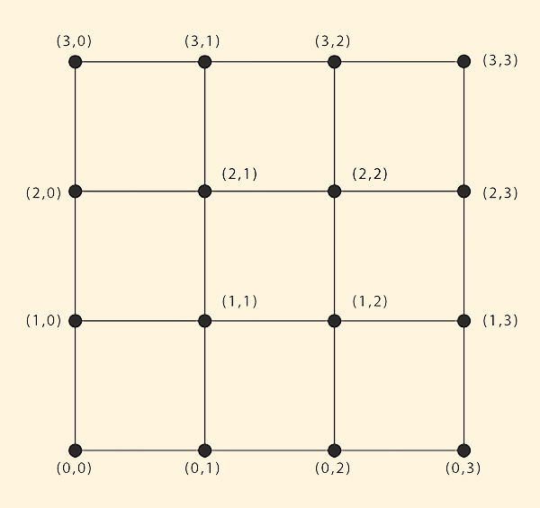
3.2 Model Components 3.2.1 Spatial Resolution The aquifer is digitally represented in plan view by means of an x-y square grid. Each interception point has an assigned grid node (x,y) as shown in Figure 3.1.
Figure 3.1 Definition sketch for square grid. The smaller the space step (Δx), the higher the spatial resolution. However, a higher resolution would have a larger number of grid nodes (x, y) and, consequently, increase the computing time required.
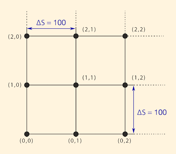
Initial testing of the model uses a 100 × 100 grid to represent an aquifer of square dimension of 10-km side dimension.
Therefore, the space
interval is
Figure 3.2 Grid configuration for model testing. 3.2.2 Aquifer Parameters
The groundwater model predicts the location of the water table, in time and space,
in two dimensions.
Depending on their vertical
position with respect to possible aquitards, aquifers may be classified
as follows: In an unconfined alluvial aquifer, the water table is at atmospheric pressure and the deposits consist of coarse alluvial materials, i.e., permeable sand and gravel. In these aquifers, the groundwater level (water table) rises and falls directly in response to external influences, such as pumping. The flow rate in porous media is directly proportional to the product of cross-sectional area and hydraulic gradient. The constant of proportionality, referred to as hydraulic conductivity K, is a quantitative measure of the capacity of the geological formation to transmit water. Hydraulic conductivity is often confused with the similar concept of permeability. Although they both convey an idea of how easily flow moves through the aquifer, they are intrinsically different. Permeability varies with temperature, pressure, and the fluid passing through the geological formation. Hydraulic conductivity, however, depends on the porosity, particle size, and distribution and arrangement of particles (Ponce, 2014). Transmissivity is a property closely related to hydraulic conductivity. It describes the rate at which water passes through a unit width of aquifer under a unit hydraulic gradient. Transmissivity T [ L2/T ] may also be defined as the product of the average hydraulic conductivity K [ L/T ] and the saturated thickness b [ L ] (Eq. 2.16). The storage coefficient S (specific yield in the case of unconfined aquifers) relates the change in hydraulic head to the change in the amount of water stored in the aquifer at a given point. It is the volume of water released from storage per unit decline in hydraulic head, per unit area. The hydraulic diffusivity v [ L2/T ] is a measure of the diffusion speed of pressure gradients in the groundwater system. It may be specified as the ratio between transmissivity T [ L2/T ] and spacific yield S (Eq. 2.17).
Tthe following values are considered for
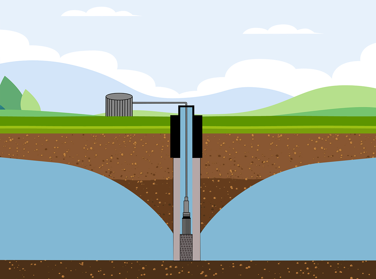
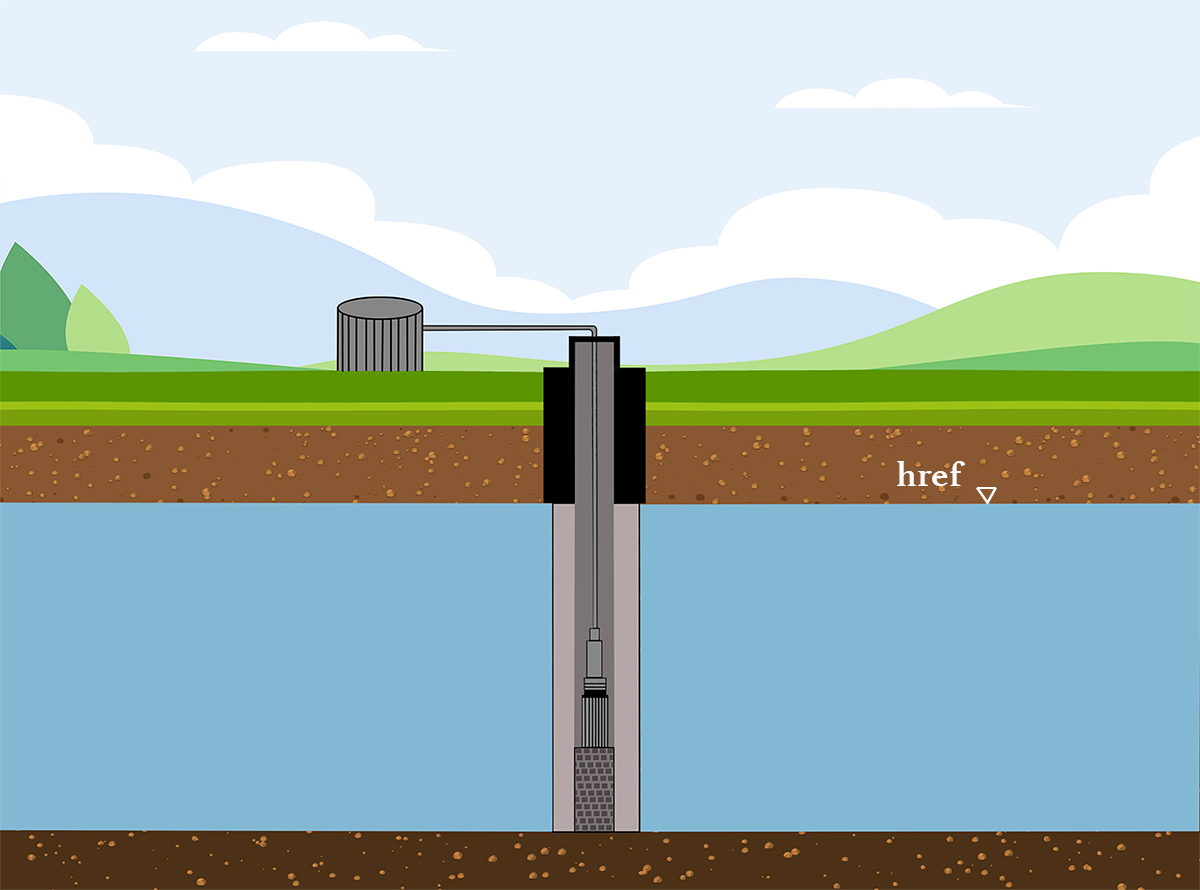
the test prototype: (a) transmissivity T = 0.01 m2 s-1, and 3.2.3 Sources and Sinks In groundwater modeling, sources constitute the entry of water into the aquifer system, such as precipitation and percolation from irrigation. Sinks are activities such as pumping, which extract (withdraw) water from the system. Withdrawal of water from an unconfined alluvial aquifer causes the groundwater level to decline in the vicinity of the withdrawal, around the pumping well. The shape of the water table becomes somewhat like an inverted cone, referred to as the cone of depression (Figure 3.3).
Figure 3.3 Cone of Depression.
The size, shape, and rate of growth of the cone of depression depends upon the following:
3.2.4 Simulation Time The model simulates the aquifer response under an uninterrupted groundwater withdrawal. Simulation time is considered to be in years. Each year is taken as 365.25 days. 3.2.5 Testing Scenarios Four different scenarios are considered, varying: (a) initial condition (steady equilibrium or non-equilibrium depleted water table), (b) presence or absence of pumping, and (c) boundary type (permeable or impermeable), as described in Table 3.1.
3.2.6 Initial Conditions The depleted water table as an initial condition (scenarios A and C) depicts a point in time when the aquifer has already been depleted by pumping. In these scenarios, the cone of depression has a depleted reference head hdref (Figure 3.4), which is an input to the model.
Figure 3.4 Reference depletion head.
The steady-equilibrium initial condition (scenarios B and D) depicts an aquifer which is about to start being pumped. The reference aquifer head href is an input of the model, which represents the initial water table elevation at the pump location (Figure 3.5).
Figure 3.5 Reference aquifer head.
Scenarios A and C, referred to as "hot-start tests", simulate aquifer recovery. For these tests,
the reference head is set at href = 500 m and the initial condition is specified as
h0 = (href - 100) in a square area of 5 km � 5 km
located in the middle of the computational
field. The aquifer bottom is set at hbottom = 0 m. Therefore,
the
Scenarios B and D, referred to as "cold-start tests", simulate aquifer depletion. For these tests,
the reference head href = 500 m is specified as initial condition at every node and the aquifer
bottom is set at hbottom = 0 m. Thus, the steady-equilibrium aquifer volume is 50,000 hm3.
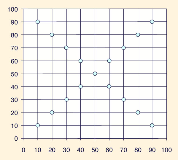
A battery of 17 pumps is symmetrically positioned across the field, at a distance of 1,414.2 m
apart, making the shape of an X (Figure 3.6). Each pump has a constant discharge of
Figure 3.6 Pump configuration for cold-start tests.
3.2.7 Boundary Type In the permeable-boundary simulation, the groundwater flows freely across the boundaries of the control volume. Aquifer depletion and recovery depend primarily on the values of the hydrogeologic properties. Impermeable boundaries impede the groundwater to move across the boundaries of the control volume. In this configuration, the depletion will occur in a relatively fast manner. The recovery will also be negatively affected, because there is no groundwater entering the system. The groundwater level may be raised only by the vertical discharge, i.e., precipitation and percolation from irrigation. 3.3 Input Description 3.3.1 Type of model In this section of the online calculator input data, one of the four scenarios described in Table 3.1 may be selected.
3.3.2 Space interval ds The space interval represents the distance between two adjacent grid points, expressed in meters. The model considers the area of the aquifer to be a square; therefore, the space interval is specified only once. The default value is ds = 100 m. 3.3.3 Number of grid intervals nz The number of grid intervals multiplied by the space interval corresponds to the length of one of the sides of the square which represents the aquifer. This is a dimensionless parameter; its default value is nz = 100. 3.3.4 Percolation from rainfall R The rainfall percolation rate is assumed to be uniformly distributed across the entire spatial domain. This parameter is expressed in mm/yr; its default value is R = 0 mm/yr. 3.3.5 Percolation from irrigation I The irrigation percolation rate is assumed to be uniformly distributed across the area defined by the user (See sections 3.3.6 and 3.3.7). The percolation from irrigation is expressed in mm/yr; its default value is I = 0 mm/yr. 3.3.6 Left location indicator for percolation from irrigation irrleft The left location indicator marks the corner grid point (on the top left) of the partial aquifer area in which the irrigation percolation rate is to be distributed. This parameter is dimensionless; its default value is irrleft = 25. 3.3.7 Right location indicator for percolation from irrigation irrright The right location indicator marks the corner grid point (on the bottom right) of the partial aquifer area in which the irrigation percolation rate is to be distributed. This parameter is dimensionless; its default value is irrright = 75. 3.3.8 Transmissivity T The aquifer transmissivity input value is expressed in units of m2/s. The default value is T = 0.01 m2/s. 3.3.9 Specific yield S The specific yield is dimensionless. The default value is S = 0.1. 3.3.10 Reference aquifer elevation href The groundwater level before pumping starts is defined as the reference aquifer elevation href, expressed in m. The default value is href = 500 m. 3.3.11 Reference depletion elevation hdref The groundwater level when pumping stops is defined as the reference depletion elevation hdref, expressed in m. The default value is hdref = 400 m. 3.3.12 Left indicator for reference depletion locleft The left location indicator marks the grid point in which the depleted aquifer area starts. As the model considers the aquifer to have a squared area, this value needs to be inputed only once. This parameter is dimentionless, and its default value is locleft = 25. 3.3.13 Right indicator for reference depletion locright The right location indicator marks the grid point in which the depleted aquifer area ends. As the model considers the aquifer to have a squared area, this value needs to be inputed only once. This parameter is dimentionless, and its default value is locleft = 75. 3.3.14 Simulation time dt
The simulation time corresponds to the time in years, during which the chosen scenario will be analyzed.
3.3.15 Printing interval tpd
As the model calculations advance, the results are printed at selected intervals.
This option allows access to not only the final result but also the
progress of the calculation.
The default value is
3.3.16 Pumping rate p
The groundwater discharge being pumped from the aquifer may be entered in this section, in units of
L/s. 3.4 Output description
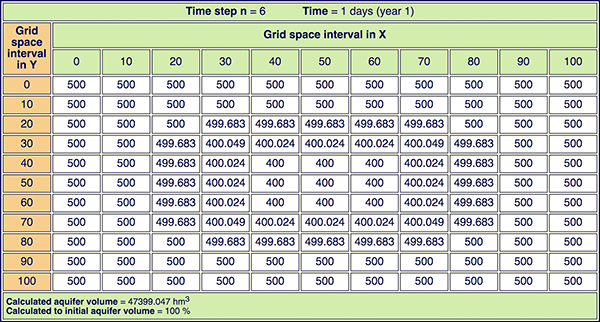
Figure 3.7 contains a sample of the model output table.
Figure 3.7 Model output table.
The number of output tables is user-defined, corresponding
to the ratio between
simulation time td and printing interval tpd. The table shows a partial, simplified version of the
complete grid, with the groundwater level values of eleven (11)
x-direction points and eleven (11) y-direction points
shown. The calculated aquifer volume and the ratio (in percentage)
between this
value and the initial aquifer volume are shown at the bottom.
4. ONLINE DEVELOPMENT
4.1 Rationale
This thesis uses the
World Wide Web as a medium to
model two-dimensional groundwater flow using a convergent explicit
finite-difference scheme.
The initial idea of the World Wide Web can be traced back to 1980,
when Tim Berners-Lee began tinkering with a software
program which he named Enquire.
The name is a short for Enquire within upon everything, a book of Victorian advice
which contained a wide range of advices, serving as
portal to a multitude of knowledge (Berners-Lee, 2000).
The original Enquire code eventually led Berners-Lee
to a vision and system
encompassing the decentralized, organic
growth of ideas, technology, and society.
Forty years after Enquire, the web has spread worldwide,
coming close to its creator's ideas of connecting anything to
anything, providing society with new freedom and faster growth.
The World Wide Web has opened up a world of possibilities,
leaving the older way of working as just one tool among many.
Created to meet the demand for automated information-sharing between scientists in universities and research institutes around
the world, the Web facilitates the disemination of information, techniques and knowledge without the physical constrains
present in the past.
Following the principle of universality and decentralization of knowledge,
the online script developed here was housed
in the World Wide Web. The script may be freely accessed
from any place at any time by anyone, requiring only a basic
understanding of groundwater flow.
The online model is written in the PHP language, which is
embedded in HTML.
The latter serves as the interface between the user and
the PHP script. The interface is designed to be highly intuitive,
therefore, eliminating the complexity typical of
other groundwater modeling software packages.
4.2 Language
The ONLINEGWMODEL.PHP was developed with the open source general-purpose
scripting language Hypertext Processor (PHP),
embedded into the Hypertext Markup Language (HTML).
In the 1980s, while working at the European Organization for Nuclear Research
(CERN),
Berners-Lee wrote a document called Information
Management: A proposal, which was the layout of his vision for what would become
eventually the World Wide Web. Only one year and a half
later, his conjoined work with Robert Cailliau included three fundamental
technologies that remain the foundation of
today's Web: HTML, URI and HTTP.
The Hypertext Markup Language (HTML) is the
standard markup language for the Web.
The Uniform Resource Identifier (URI)
is a string of characters that identifies a particular resource, following
predefined syntax rules.
The Hypertext Transfer Protocol (HTTP) is an application
protocol for distributed, collaborative, hypermedia
information systems, allowing for the retrieval
of linked resources from across the Web.
HTML was strongly based on SGML (Standard Generalized Markup Language), an
internationally agreed upon method for marking up text
into structural units such as paragraphs, headings and list
items. Berners-Lee's major
contribution was the hypertext link,
the idea of using the anchor element a
with the href
attribute.
The language is independent of the formatter, subsequently referred to as the
browser,
which displays the text on the screen.
Over the years since its initial development,
HTML went through a series of improvements in a joint effort by academics and computer
scientists from all around the world. The current version is HTML 5.0, dated 2012.
The Hypertext processor (PHP) is an HTML-embedded server-side scripting language.
In 1994, Rasmus Lerdorf started what would
become the PHP language using a simple set of Common Gateway Interface (CGI)
binaries written in the C programming
language. In 1995, Lerdorf released the code source to
the public, allowing developers to use it and improve it.
Many versions of the code followed as PHP gained in
popularity around the world.
In 1997, Andi Gutmans and Zeev Suraski started collaborating with Lerdorf in the
development of a new, independent programming language, which eventually evolved into a scripting language based on C,
Java, and Perl. The current version is PHP 7.4.5, dated 2020.
The script runs on the user's server, requiring a PHP parser, a web server, and a web
browser. The PHP code is analyzed using the PHP parser,
and the server makes the output viewable on the web page in
the web browser. Scripts can also be used with command line scripting, in which a server and web browser are not
required to execute the code, but simply the PHP parser (Achour et al. 2014).
Both PHP and HTML code can be interpreted by PHP files;
thus, allowing the files to swap between languages. Once
the PHP code is executed on the server, an HTML file
is generated to be viewed by the user, while masking the code
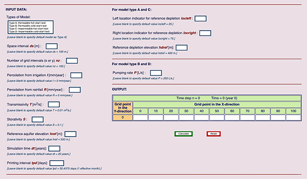
(Achour et al. 2014). In ONLINEGWMODEL.PHP, the input cell
were developed using HTML (Figure 4.1).
PHP interprets the input values and runs the code
to compute the aquifer elevation throughout the grid.
The output tables (Figure 3.7) are also developed using HTML, allowing the interpretation of the
model's output.
[Click on the image to display larger size]
Figure 4.1 ONLINEGWMODEL.PHP data input display.
4.3 Convergence Testing
Ponce et al. (2001)
tested the numerical model for
the four scenarios described in Table 3.1.
ONLINEGWMODEL.PHP was tested under similar conditions, using a
reference head href = 500 m.
[Click on the image to display larger size]
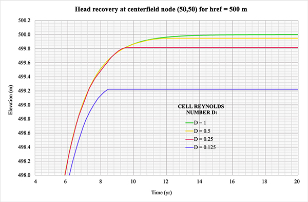
Figure 4.2 Head recovery at centerfield node (50,50) for href = 500 m.
The convergence testing of ONLINEGWMODEL.PHP is seen to reproduce the findings of
Ponce et al. (2001). The conclusion is that the explicit groundwater model
is convergent only for cell Reynolds number D = 1.
5. MODEL APPLICATION
A hypothetical square aquifer with the parameters described in Table 5.1
was used to test ONLINEGWMODEL.PHP under four
different conditions (scenarios A to D):
The four scenarios considered were modeled for a total simulation time of 20 years.
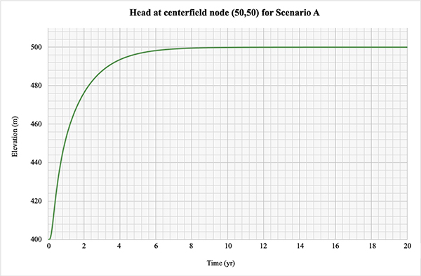
5.1 Scenario A: Permeable hot-start test
This scenario assesses aquifer recovery under a permeable boundary,
following depletion by pumping. The equilibrium aquifer elevation is
500 m, corresponding to an aquifer volume of
The piezometric level returned to steady-equilibrium condition (exactly h = 500 m at every node) in an asymptotic fashion after
18.67 yr. simulation (Figure 5.1).
The calculated aquifer volume at
the end of the simulation is
[Click on the image to display larger size]
Figure 5.1 Head at centerfield node (50,50) for permeable hot-start test.
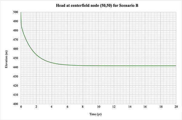
5.2 Scenario B: Permeable cold-start test
This scenario assesses aquifer depletion as a consequence of pumping, under a permeable boundary.
A battery of 17 pumps symmetrically positioned
across the field is specified, with a pumping rate of 250 L/s per
pump.
Initially, the aquifer elevation is specified at 500 m in every node,
corresponding
to an aquifer volume of 50,000 hm3.
With ongoing pumping, eventually
the piezometric level reached a steady-equilibrium condition, with the
maximum depletion level (h = 441.644 m) at the
centerfield node (50,50).
The calculated aquifer volume, at equilibrium after depletion,
is 48,217.36 hm3.
The final volume, in percentage, calculated by taking the initial aquifer
volume, subtracting the pumped volume and adding the boundary inflows, is equal to
96.435% at the end of the 20-yr simulation.
The model is shown to be strongly stable.
[Click on the image to display larger size]
Figure 5.2 Head at centerfield node (50,50) for permeable cold-start test.
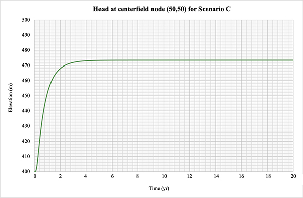
5.3 Scenario C: Impermeable hot-start test
This scenario assesses aquifer recovery under an impermeable boundary,
following depletion by pumping.
The equilibrium aquifer elevation is
500 m, corresponding to a total aquifer volume of 50,000 hm3.
The initial depletion is specified in a
square grid located in the center of the model, from
grid point No. 25 to grid point No. 75.
The reference depletion elevation is 400 m, corresponding
to an initial aquifer volume of 47,399 hm3.
The piezometric level returned to steady-equilibrium condition (h = 473.462 m at every node) in an
asymptotic
fashion after 9.58 yr. simulation (Figure 5.3).
The calculated aquifer volume is 47,346 hm3,
which corresponds to 99.89 percent of volume conservation, that is,
a 0.11 percent of numerical loss of mass.
The model is shown to be strongly stable.
[Click on the image to display larger size]
Figure 5.3 Head at centerfield node (50,50) for impermeable hot-start test.
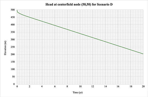
5.4 Scenario D: Impermeable cold-start test
This scenario assesses aquifer depletion as a consequence of pumping,
under an impermeable boundary.
A battery of 17 pumps symmetrically positioned
across the field is specified, with a pumping rate of 250 L/s per pump.
Initially, the aquifer elevation is specified at 500 m in every node,
corresponding
to an initial aquifer volume of 50,000 hm3.
The piezometric level decreased in a linear fashion, with the maximum
depletion (h = 203.894 m) at the centerfield node (50,50) after 20 yr of simulation, correctly simulating the linear depletion of
the aquifer under Scenario D, i.e., with
pumping under an impermeable boundary (Figure 5.4).
[Click on the image to display larger size]
Figure 5.4 Head at centerfield node (50,50) for impermeable cold-start test.
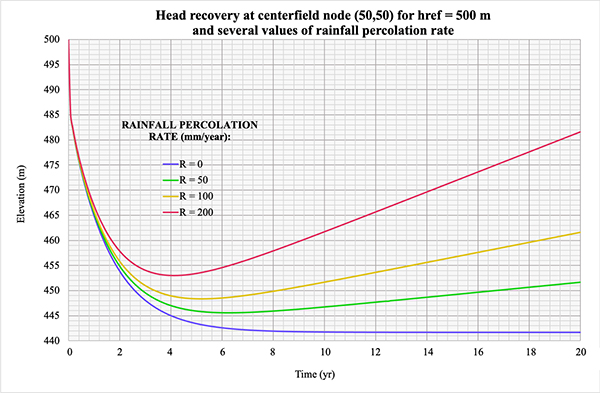
5.5 Percolation from rainfall
The model was tested to simulate percolation originating in rainfall.
The model assumes a uniform spatial distribution of
precolation from rainfall across the spatial domain.
Scenario B was chosen for this purpose.
The input to the model is the same as that described in Section 5.2.
Four tests were performed considering the following
values of rainfall percolation rate:
[Click on the image to display larger size]
Figure 5.5 Head recovery at centerfield node (50,50) for href = 500 m
When there is no percolation from rainfall, the cone of depression reaches an equilibrium elevation of 441.66 m
in an asymptotic fashion after 17.67 yr. of simulation. When rainfall percolation is present, the cone of depression
does not reach equilibrium conditions. As the simulation progresses, the aquifer elevation reaches a minimum value,
after which it begins to increase.
For a rainfall percolation rate equal to 50 mm/yr,
the aquifer elevation reaches a minimum value of 445.543 m after 6.24 yr of simulation.
From this point on, the aquifer elevation increases gradually, reaching 451.626 m at the end of the simulation.
For a rainfall percolation rate equal to 100 mm/yr,
the aquifer elevation reaches a minimum value of 448.373 m after 5.24 yr of simulation.
From this point on, the aquifer elevation increases gradually, reaching 461.608 m at the end of the simulation.
For a rainfall percolation equal to 200 mm/yr,
the aquifer elevation reaches a minimum value of 452.965 m after 4.07 yr of simulation.
From this point on, the aquifer elevation increases gradually, reaching 481.571 m in the end of the simulation.
As expected, the results show that the greater the rainfall percolation rate:
(1) the less accentuated is the minimum value of aquifer elevation, and (2)
the higher the aquifer elevation at the end of the simulation time.
In conclusion, the model is shown to satisfactorily represent
the aquifer response in the presence of percolation from rainfall.
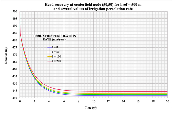
5.6 Percolation from irrigation
The model was tested to simulate percolation originating in irrigation. Scenario B was chosen for this purpose.
By default, the percolation from irrigation is uniformly distributed in a square area
of
[Click on the image to display larger size]
Figure 5.6 Head recovery at centerfield node (50,50) for href = 500 m
In contrast to the case of percolation from rainfall, the aquifer elevation
due to percolation from irrigation reaches an equilibrium value.
For the percolation rate equal to 0 mm/yr, the aquifer elevation reaches an equilibrium level of
441.644 m in an asymptotic fashion after 6.24 yr of simulation.
For the percolation rate equal to 50 mm/yr,
the aquifer elevation reaches an equilibrium level of 442.365 m
in an asymptotic fashion after 8.98 yr
of simulation.
For the percolation rate equal to 100 mm/yr, the aquifer elevation reaches an equilibrium level
of 443.085 m in an asymptotic fashion after 9.23 yr of simulation.
For the percolation rate equal to 200 mm/yr,
the aquifer elevation reaches an equilibrium level of 444.526 m
in an asymptotic fashion after 9.81 yr of simulation.
As expected, the results show that the greater the irrigation percolation rate, the higher the aquifer
elevation at the end of the simulation time. In conclusion, the model is shown to satisfactorily represent
the aquifer response in the presence of percolation from irrigation.
The fact that the cone of depression
does not reach equilibrium
conditions in the case of rainfall percolation,
but it reaches it
in the case of irrigation percolation
may be attributed, in part, to the marked difference in
specified spatial distributions.
6. SUMMARY AND CONCLUSIONS
6.1 Summary
The convergent explicit groundwater flow model presented by
Ponce et al. (2001) in the FORTRAN language was converted
into the PHP language and adapted for online use.
The model may be freely accessed by anyone from any place at any time,
requiring only a basic understanding of groundwater flow. The simplicity of its
structure and operation, coupled with its strong stability and convergence properties,
makes the model particularly suited
for the online teaching and learning of groundwater flow modeling.
The numerical model is an explicit formulation of the two-dimensional (x-y) diffusion equation of flow in porous media,
applicable to a homogeneous isotropic aquifer. Explicit models are subject to a
stability criterion in order to
remain stable. As shown here,
the numerical model must also satisfy a convergence criterion to preserve accuracy.
The satisfaction of both
stability and convergence requires that the cell Reynolds number D = 1.
The online groundwater model uses a simplified representation of an
aquifer to simulate its behavior under
four types of aquifer use. The input data consists of the following:
(1) aquifer geometry (aerial dimensions and depth); (2) aquifer
properties (transmissivity and specific yield);
and (3) discretization data (space step and total
simulation time). The time step is internally defined following the
condition cell Reynolds number D = 1.
Testing of the model under several hypothetical conditions showed that
the model is stable, convergent, and numerically mass conservative.
Testing of rainfall and irrigation percolation are also shown to be
in agreement with the governing equations.
Overall, the tests show that the modeling of
groundwater flow using ONLINEGWMODEL.PHP is well
behaved and properly responsive to variations in input parameters.
6.2 Conclusions
Testing of the model under hypothetical conditions showed
that the model is stable, convergent, and numerically mass conservative.
The permeable hot-start test converged to the steady-equilibrium baseline condition after 15.85 yr. The permeable
cold-start test converged to a steady-equilibrium cone of depression after 12.43 yr. The impermeable hot-start test
converged to a steady-equilibrium non-baseline condition after 8.34 yr. The impermeable cold-start test properly
simulated the linear depletion of the aquifer.
The condition cell Reynolds number D = 1 is shown to properly and effectively
guarantee that the model will be stable,
convergent, and consistent with the governing differential equations used in its formulation.
This property makes the model particularly suited for online teaching and
learning
of groundwater flow modeling and behavior.
6.3 Recommendations
The model presented herein
was developed to test aquifer depletion and recovery
under several specifications of boundary type,
on/off pumping, and initial conditions. For simplicity,
to reduce the number of input parameters,
the model uses a square-grid configuration.
It is recommended
that the model be further extended to
handle a complex spatial specification, aquifer anisotropy, and confined aquifers.
REFERENCES
Achour, M., F. Betz, A. Dovgal, N. Lopes, H. Magnusson, G. Richter, D. Seguy, and J. Vrana.
"PHP Manual." Edited by Philip Olson. (2014).
Berners-Lee, Tim. "Weaving The Web: the Original Design and Ultimate Destiny of the World Wide
Web by Its Inventor." New York: HarperCollins Publishers, 2000.
Chow, V.T. "Open Channel Hydraulics." New York: McGraw-Hill (1959).
Cunge, J. A. "On the Subject of a Flood Propagation Computation Method (Musklngum Method)."
Journal of Hydraulic Research 7, no. 2 (1969): 205-30.
Douglas, J. "On the Relation between Stability and Convergence in the Numerical Solution of
Linear Parabolic and Hyperbolic Differential Equations." Journal of the Society for Industrial
and Applied Mathematics 4, no. 1 (1956): 20-37.
Freeze, R. A., and J. A. Cherry. "Groundwater." Englewood Cliffs, NJ: Prentice-Hall (1979).
Gary, J. "The Numerical Solution of Partial Differential Equations." National Center for Atmospheric Research no. 69-54 (1969).
Jain, S. K., and V. P. Singh. "Chapter 11 - Reservoir Operation."
In Developments in Water Science, edited by S. K. Jain and V. P. Singh, 615-79: Elsevier (2003).
Kresic, N. "Quantitative Solutions in Hydrogeology and Groundwater Modeling." New York: Lewis (1997).
Langevin, C. D., and S. Panday. "Future of Groundwater Modeling." Groundwater 50, no. 3 (2012): 334-39.
Lomax, H., T. H. Pulliam and Zingg, D. "Fundamentals of Computational Fluid Dynamics." Germany: Springer-Verlag (2001).
Malcherek, A. and W. Zielke. "Upwinding and Characteristics in FD and FE Methods."
Computer Modeling of Free-Surface and Pressurized Flows. Germany: Kluwer Academic Publishers (1994).
National Research Council. " Models in Environmental Regulatory Decision Making." Committee on
Models in the Regulatory Decision Process . Washington, DC: National Academies Press (2007).
O'Brien, G. G., M. A. Hyman, and S. Kaplan." A Study of the Numerical Solution of Partial
Differential Equations." Journal of Mathematics and Physics 29, no. 1-4 (1950): 223-51.
Ponce, V. M., R. M. Li and D. B. Simons. "Applicability of Kinematic and Diffusion Models."
Journal of the Hydraulics Division, ASCE, no. 104(HY3) (1978): 353-60.
Ponce, V. M., H. Indlekofer, and D. B. Simons. "Convergence of Four-Point Implicit Water Wave Models."
Journal of the Hydraulics Division, ASCE, no. 104(HY7) (1978): 947-58.
Ponce, V. M, H. Indlekofer, and D. B. Simons. "The Convergence of Implicit Bed Transient Models."
Journal of the Hydraulics Division, ASCE, no. 105(HY4) (1979): 351-63.
Ponce, V. M., A. Shetty, and A. Ercan. "A Convergent Explicit Groundwater Model." Online article. (2001).
Ponce, V. M.
"Engineering Hydrology: Principles and Practices."
Second edition, online (2014).
Ravazzani, G., D. Rametta, and M. Mancini. "Macroscopic Cellular Automata for Groundwater Modelling:
A First Approach." Environmental Modelling & Software 26, no. 5 (2011/05/01/ 2011): 634-43.
Refsgarrd, J. C., A. L. Hojberg, I. Moller, M. Hansen, and V. Sondergaard.
"Groundwater Modeling in Integrated Water Resources Management - Visions for 2020."
Groundwater 48, no. 5 (2010): 633-648.
Reilly, T. E., K. F. Dennehy, W. M. Alley, and W. L. Cunningham.
"Ground-Water Availability in the United States." Geological Survey (2008).
Roache, P. J. "Computational Fluid Dynamics." Albuquerque, NM: Hermosa Publishers (1972).
Rushton, K. R., and S. C. Redshaw. Seepage and Groundwater Flow,
"Numerical Analysis by Analog and Digital Methods. Earth Surface Processes."
Vol. 5, New York: John Wiley & Sons (1980).
Zheng, C. "Reflections: 2002-2010." Groundwater 49, no. 2 (2011): 129-132.
|
|||||||||||||||||||||||||||||||||||||||||||||||||||||||||||||||||||||||||||||||||||||||||||||||||||||||||||||||||||||||||||||||||||||||||||||||||||||||||||||||||||||||||||||||||||||||||||||||||||||||||||||||||||||||||||||||||||||||||||||||||||||||||||||||||||||||||||||||||||||||||||||||||||||||||||||||||||||||||||||||||||||||||||||||||||||||||||||||||||||||||||||||||||||||||||||||||||||||||||||

| 800 px ruler |