APPLICATION OF THE GENERAL DIMENSIONLESS UNIT HYDROGRAPH USING CALIFORNIA WATERSHED DATA
Luis Gustavo Ariza Trelles
1. INTRODUCTION
1.1 Introduction The concept of unit hydrograph is well established in hydrologic engineering research and practice. The unit hydrograph is defined as the hydrograph produced by a unit depth of runoff uniformly distributed over the entire catchment (watershed or basin) and lasting a specified unit duration. The concept has been used since the 1930s for the simulation of flood flows around the world (Sherman, 1932). The general dimensionless unit hydrograph (GDUH), developed by Ponce (2009a, 2009b), is a dimensionless formulation of the unit hydrograph. The GDUH effectively associates the convolution technique (of the unit hydrograph) with the model of cascade of linear reservoirs (CLR), originally due to Nash (1957). The CLR model constitutes the routing component of several hydrologic models that have since been developed around the world, notably the SSARR model (U.S. Army Engineer North Pacific Division, 1972). This study attempts to validate the GDUH model using California watershed/basin data. Geographic and rainfall-runoff data is readily available online in the State of California, thus facilitaling collection and analysis. Digital elevation maps (DEM) are available from the USGS virtual platforms Earth Explorer and Alaska Satellite Facility. Rainfall data is available from the NOAA virtual platform National Centers for Environmental Information. Runoff data is available from the USGS virtual platform National Water Information System. This study selects ten (10) California watersheds/basins for analysis. To enable the proper study of unit hydrograph diffusion, the basins encompass a wide range in the values of geomorphological parameters (drainage area, average land surface slope, and stream channel slope). Conceptual and statistical analyses are used to develop a methodology for the accurate prediction of unit hydrographs on the basis of local/regional geomorphology. Given the prospect of global warming and its magnifying effect on flood flows, the timeliness of this endeavor cannot be overemphasized. 1.2 Objectives The objectives of this study are: General
Specific
1.3 Scope This study encompasses the development and validation of a predictive methodology to calculate unit hydrographs based on local/regional geomorphology. The avowed strength of the methodology is its conceptual basis, being based on time-tested cascade of linear reservoirs theory. The central focus on the general dimensionless unit hydrograph (GDUH) as a unifying theory enhances the validation exercise.
2. BACKGROUND
2.1 The unit hydrograph Over the past century, the unit hydrograph (UH) has been used as a methodology to generate flood flows for midsize and large basins (Ponce, 1989; Ponce, 2014a). In 1930, the Committee on Floods of the Boston Society of Civil Engineers, after a study of New England flood hydrographs, concluded the following (referenced by Hoyt et. al., 1936, p. 123):
This statement may be interpreted as follows: For a certain basin of drainage area A, given a single rainfall event of effective depth d and duration tr, which covers the entire area, the volumen of runoff Vr and consequently the peak flow Qp, are proportional to the effective rainfall intensity d/tr. In other words, the hydrograph response (Q) is linear with respect to the intensity and, therefore, independent of the time base Tb. Sherman (1932) built on this concept to develop the unit hydrograph for flood studies in large basins. The word unit is normally understood to refer to a unit depth of effective rainfall or runoff. However, it should be noted that Sherman first used the word to describe a unit depth of runoff (1 cm or 1 in.) lasting a unit increment of time, i.e., an indivisible increment. The unit increment of time can be either 1-h, 3-h, 6-h, 12-h, 24-h, or any other suitable duration (Ponce, 2014a). The unit hydrograph is defined as the hydrograph produced by a unit depth of runoff uniformly distributed over the entire catchment (watershed or basin) and lasting a specified unit duration. To illustrate the concept of unit hydrograph, assume that a certain storm produces 1 cm of runoff and covers a 50-km2 catchment over a period of 2 h. The hydrograph measured at the catchment outlet would be the 2-h unit hydrograph for this 50-km2 catchment (Fig. 2.1).
Two assumptions are crucial to the development of the unit hydrograph: (1) linearity, and
The time base of all hydrographs obtained in this way is equal to that of the unit hydrograph. Therefore, the procedure can be used to calculate hydrographs produced by a storm consisting of a series of runoff depths, each lagged in time one increment of unit hydrograph duration, as shown in Fig. 2.2 (b).
The summation of the corresponding ordinates of these hydrographs (superposition) allows the calculation of the composite hydrograph, as shown in Fig. 2.2 (c). The procedure depicted in Fig. 2.2 is referred to as the convolution of a unit hydrograph with an effective storm pattern (hyetograph). In essence, the procedure amounts to stating that the composite hydrograph ordinates are a linear combination of the unit hydrograph ordinates.
The assumption of linearity has long been considered one of the limitations of unit hydrograph theory. In nature, it is unlikely that catchment response will always follow a linear function. For one thing, discharge and mean velocity are nonlinear functions of flow depth and stage. In practice, however, the linear assumption provides a convenient means of calculating runoff response without the complexities associated with nonlinear analysis. The upper limit of applicability of the unit hydrograph is not very well defined. Sherman (1932) used it in connection with basins varying from 1300 to 8000 km2. Linsley et. al. (1962) mention an upper limit of 5000 km2 in order to preserve accuracy. More recently, the unit hydrograph has been linked to the concept of midsize catchment, i.e., greater than 2.5 km2 and less than 250 km2. This certainly does not preclude the unit hydrograph technique from being applied to catchments larger than 250 km2, although overall accuracy is likely to decrease with an increase in catchment size (Ponce, 2014a). 2.2 Storage routing and linear reservoirs As shown in Section 2.3, the concepts of unit hydrograph and cascade of linear reservoirs are intrinsically connected. The cascade is effectively a series of linear reservoirs, and the latter is a way of performing storage routing. Therefore, this section addresses storage routing and linear reservoirs. The techniques for storage routing are invariably based on the differential equation of water storage. This equation is founded on the principle of mass conservation, which states that the change in flow per unit length in a control volume is balanced by the change in flow area per unit time. In partial differential form it is expressed as follows:
in which Q = flow rate, A = flow area, x = space (length), and t = time. The differential equation of storage is obtained by lumping spatial variations. For this purpose, Eq. 2-1 is expressed in finite increments:
With ΔQ = O - I, in which O = outflow and I = inflow; and ΔS = ΔA Δx , in which ΔS = change in storage volume, Eq. 2-2 reduces to:
in which inflow, outflow, and rate of change of storage are expressed in
L3T -1 units.
Furthermore,
Equation 2-4 implies that any difference between inflow and outflow is balanced by a change of storage in time (Fig. 2.3). In a typical reservoir routing application, the inflow hydrograph (upstream boundary condition), initial outflow and storage (initial conditions), and reservoir physical and operational characteristics are known. Thus, the objective is to calculate the outflow hydrograph for the given initial condition, upstream boundary condition, reservoir characteristics, and operational rules.
Equation 2-4 can be solved by analytical or numerical means. The numerical approach is usually preferred because it can account for an arbitrary inflow hydrograph. The solution is accomplished by discretizing Eq. 2-4 on the x-t plane, a graph showing the values of a certain variable in discrete points in time and space (Fig. 2.4). Figure 2.4 shows two consecutive time levels, 1 and 2, separated between them an interval Δt, and two spatial locations depicting inflow and outflow, with the reservoir located between them. The discretization of Eq. 2-4 on the x-t plane leads to:
in which I1 = inflow at time level 1; I2 = inflow at time level 2; O1 = outflow at time level 1; O2 = outflow at time level 2; S1 = storage at time level 1; S2 = storage at time level 2; and Δt = time interval. Equation 2-5 states that between two time levels 1 and 2 separated by a time interval Δt, average inflow minus average outflow is equal to change in storage (Ponce, 2014a).
For linear reservoirs, the relation between storage and outflow is linear. Therefore:
and
in which K = storage constant, in T units. Substituting Eqs. 2-6 into 2-5, and solving for O2:
in which C0, C1 and C2 are routing coefficients defined as follows:
Since C0 + C1 + C2 = 1, the routing coefficients are interpreted as weighting coefficients. These routing coefficients are a function of Δt /K, the ratio of time interval to storage constant. Values of the routing coefficients as a function of Δt /K are given in Table 2.1.
A reservoir exerts a diffusive action on the flow, with the net result that the peak flow is attenuated and
consequently, the time base is increased.
For the case of a linear reservoir, the amount of attenuation is a function of 2.3 The cascade of linear reservoirs
The cascade of linear reservoirs is a widely used method of hydrologic catchment routing.
As its name implies, the method is based on the connection of several linear reservoirs in series.
For N such reservoirs, the outflow from the first would be taken as inflow to the second, the
outflow from the second as inflow to the third, and so on, until the outflow from the
(N - 1)th reservoir, is taken as inflow to the Each reservoir in the series provides a certain amount of diffusion and associated lag. For a given set of parameters Δt/K and N, the outflow from the last reservoir is a function of the inflow to the first reservoir. In this way, a one-parameter linear reservoir method (Δt/K) is extended to a two-parameter catchment routing method. The addition of the second parameter (N) provides considerable flexibility in simulating a wide range of diffusion and associated lag effects. The method has been widely used in catchment simulation, primarily in applications involving large gaged river basins. Rainfall-runoff data can be used to calibrate the method, i.e., to determine a set of parameters Δt/K and N that produces the best fit to the measured data.
The solution of the cascade of linear reservoirs can be accomplished in two ways: (1) analytical, and (2) numerical.
The analytical version is due to The numerical version of the cascade of linear reservoirs is featured in several hydrologic simulation models developed in the United States and other countries. Notable among them is the Streamflow Synthesis and Reservoir Regulation (SSARR) model, which uses it in its watershed, stream channel routing, and baseflow modules. The SSARR model has been in the process of development and application since 1956. The model was developed to meet the needs of the U.S. Army Corps of Engineers North Pacific Division in the area of mathematical hydrologic simulation for planning, design, and operation of water-control works. (U.S. Army Engineer North Pacific Division, 1972). The SSARR model was first applied to operational flow forecasting and river management activities in the Columbia River System. Later, it was used by U.S. Army Corps of Engineers, National Weather Service, and Bonneville Power Administration. Numerous river systems in the United States and other countries have been modeled with SSARR. To derive the routing equation for the method of cascade of linear reservoirs, Eq. 2-7 is reproduced here in a slightly different form:
in which Q represents discharge, whether inflow or outflow and j and n are space and time indexes, respectively (Fig. 2.5).
As with Eq. 2-7, the routing coefficients C0, C1 and C2
are a function of the dimensionless ratio
For application to catchment routing, it is convenient to define the average inflow as follows:
Substituting Eqs. 2-10b and 2-11 into Eq. 2-9 gives the following:
or, alternatively, through some algebraic manipulation:
Equations 2-12 and 2-13 are in a form convenient for catchment routing because the inflow is usually a rainfall hyetograph, that is, a constant average value per time interval. Note that Eqs. 2-12 and 2-13 are identical. Equation 2-12 was presented by Ponce in his version of the cascade of linear reservoirs (Ponce, 2014a). Equation 2-13 is the routing equation of the SSARR model (U.S. Army Engineer North Pacific Division, 1972).
Smaller values of C lead to greater amounts of runoff diffusion.
For values of C > 2, the behavior of Eq. 2-12 (or Eq. 2-13) is highly dependent on the type of input.
For instance, in the case of a unit impulse (rainfall duration equal to the time interval), Eq. 2-12 The cascade of linear reservoirs provides a convenient mechanism for simulating a wide range of catchment routing problems. Furthermore, the method can be applied to each runoff component (surface runoff, subsurface runoff, and baseflow) separately, and the catchment response can be taken as the sum of the responses of the individual components.
For instance, assume that a certain basin has 10 cm of runoff, of which 7 cm are surface runoff, 2 cm are subsurface runoff, and 1 cm is baseflow.
Since surface runoff is the less diffused process, it can be simulated with a high Courant number, say C = 1, and a small number of reservoirs, say N = 3.
Subsurface runoff is much more diffused than surface runoff; therefore, it can be simulated with C = 0.4 and N = 5.
Baseflow, being very diffused, can be simulated with C = 0.1 and N = 7 2.4 The instantaneous unit hydrograph
According to Nash, the general equation for the instantaneous unit hydrograph is:
in which u = unit hydrograph ordinate, and t = time.
In this equation: V = unit hydrograph volume; Equation 2-14 is the analytical version of the IUH or cascade of linear reservoirs. The numerical version is represented by either Ponce's model (Eq. 2-12) or the SSARR model (Eq. 2-13). 2.5 The geomorphologic instantaneous unit hydrograph Rodríguez-Iturbe and Valdés (1979) pioneered in establishing the relation of the instantaneous unit hydrograph with the geomorphologic characteristics of the catchment; see also the companion papers (Valdés et. al. 1979; Rodríguez-Iturbe et. al. 1979). The geomorphologic characteristics are expressed in terms of the following basin parameters:
According to Rodríguez-Iturbe and Valdés (1979), the equations to calculate the geomorphologic instantaneous unit hydrograph (GIUH) are:
In which qp = peak discharge, in T -1 units; and tp = time-to-peak, in T units. The parameters θ and k are a function of the basin parameters RA, RB, RL, and LΩ, as follows:
The parameters θ and k have dimensions of L -1 and L, respectively. Equations 2-18 and 2-19 assume the basin order Ω = 3, and the hydraulic length of the first-order subbasin L1 = 1000 m. 2.6 The concept of runoff diffusion
The unit hydrograph seeks to calculate runoff diffusion, i.e., the spreading of the hydrograph in time and space.
In practice, the amount of runoff diffusion depends on whether the flow is through: (a) a reservoir, Flow through a reservoir always produces runoff diffusion. Flow in stream channels may or may not produce runoff diffusion, depending on the relative scale of the flood wave, provided the Vedernikov number is less than 1. The relative scale of the flood wave relates to whether the wave is: (a) kinematic, (b) diffusion, or (c) mixed kinematic-dynamic. In catchment flow, diffusion is produced: (1) for all wave types, when the time of concentration exceeds the effective rainfall duration, or (2) for all effective rainfall durations, when the wave is a diffusion wave (Ponce, 2014b). 2.6.1 Runoff diffusion in reservoirs Reservoirs are natural or artificial surface-water hydraulic features that provide runoff diffusion. Runoff diffusion is depicted by the sizable attenuation of the inflow hydrograph, as shown in Fig. 2.6.
2.6.2 Runoff diffusion in stream channels Stream channels, i.e., channels or canals, are surface-water hydraulic features which may or may not provide runoff diffusion, depending on the relative scale of the disturbance (flood wave). The amount of wave diffusion is characterized by the dimensionless wavenumber σ, as shown in Fig. 2.7. The dimensionless wavenumber is defined as:
in which L = wavelength of the disturbance, and Lo = the length of channel in which the equilibrium flow drops a head equal to its depth (Lighthill and Whitham, 1955):
Four types of waves are identified:
Kinematic waves lie on the left side of the wavenumber spectrum, featuring constant dimensionless relative wave celerity and zero attenuation. Dynamic waves lie on the right side, featuring constant dimensionless relative wave celerity and zero attenuation. Mixed kinematic-dynamic waves lie in the middle of the spectrum, featuring variable dimensionless relative wave celerity and medium to high attenuation. Diffusion waves are intermediate between kinematic and mixed kinematic-dynamic waves, featuring mild attenuation. In hydraulic engineering practice, dynamic waves are commonly referred to as Lagrange or "short" waves, while the mixed kinematic-dynamic waves are commonly referred to as "dynamic waves," fueling a semantic confusion.
For flood routing computations, the governing equations of continuity and motion, commonly referred to as the Saint Venant equations, may be linearized and combined into a convection-diffusion equation with discharge Q as the dependent variable (Hayami, 1951; Dooge, 1973; Dooge et al., 1982; Ponce, 1991a ; Ponce, 1991b):
in which V = Vedernikov number, defined as the ratio of relative kinematic wave celerity to relative dynamic wave celerity (Ponce, 1991b):
in which β = exponent of the discharge-flow area rating Q =
In Eq. 2-22, for V = 0, the coefficient of the second-order term reduces
to the kinematic hydraulic diffusivity, originally due to
Hayami (1951).
On the other hand, for V = 1, the coefficient of the second-order term reduces to zero,
and the diffusion term vanishes. Under this latter flow condition, all waves, regardless of scale,
travel with the same speed, fostering the development of roll waves (Fig. 2.8).
Fig. 2.8 Roll waves in a steep canal, Cabana-Mañazo irrigation, Puno, Peru.
2.6.3 Runoff diffusion in catchments
Surface runoff in catchments may be one of three types
(Ponce, 1989a; 2014a):
Concentrated flow, when the effective rainfall duration is equal to the time of concentration,
Superconcentrated flow, when the effective rainfall duration is longer than the time of concentration, and
Subconcentrated flow, when the effective rainfall duration is shorter than the time of concentration.
Figure 2.9 shows a typical open-book schematization for
overland flow modeling. Input is effective rainfall on two planes adjacent ot a channel.
Output is the outflow hydrograph at the catchment outlet.
Fig. 2.9 Open-book catchment schematization.
Figure 2.10 shows dimensionless catchment outflow hydrographs for the three cases described above
(Ponce and Klabunde, 1999).
The maximum possible peak outflow is: Qp = Ie A,
in which Ie = effective rainfall intensity, and A = catchment area.
By definition, the maximum possible peak outflow is reached for
superconcentrated and concentrated flow.
However, in the case of subconcentrated flow, the peak outflow fails to reach the maximum possible value. Effectively, this
amounts to runoff diffusion, because the flow has actually been spread in time (and space).
Thus, runoff diffusion is produced for all waves
when the time of concentration exceeds the effective rainfall duration.
This is typically the case of midsize and large basins, for which the
catchment slope (along the hydraulic length) is sufficiently mild (small).
The time of concentration is directly related to catchment hydraulic length and bottom friction,
and inversely related to bottom slope and
effective rainfall intensity (Ponce, 1989b;
2014b).
Fig. 2.10 Dimensionless catchment runoff hydrographs (Ponce and Klabunde, 1999).
Figure 2.11 shows dimensionless rising overland flow hydrographs for a kinematic wave model (labeled KW)
and for several storage-concept models,
for the discharge-area rating exponent m ranging from m = 1, corresponding to a
linear reservoir, to m = 3, corresponding to laminar flow
(Ponce et al., 1997). The kinematic wave time-to-equilibrium,
akin to the time of concentration, is theoretically equal to one-half
of the time of concentration of the storage-based models
(Ponce, 1989;
2014).
It is seen that the storage models spread the hydrograph and, consequently, produce diffusion, while the
kinematic wave model lacks runoff diffusion altogether. The kinematic time-to-equilibrium is the shortest possible value
of time of concentration, resulting, in the aggregate, in the largest peak flows.
Thus, under pure kinematic flow, runoff diffusion vanishes.
Fig. 2.11 Dimensionless rising hydrographs of overland flow (Ponce et al., 1997).
In actual numerical computations, a kinematic wave model may not be entirely devoid of diffusion, due to the appearance
of numerical diffusion (Cunge, 1969; Ponce, 1991a). In fact, first-order schemes of the kinematic wave equation produce numerical diffusion.
This diffusion, however, is uncontrolled, not based on physical parameters and, therefore, unrelated to the true
diffusion of the physical problem.
2.7 The general dimensionless unit hydrograph
The cascade of linear reservoirs (CLR) (Section 2.3) and the instantaneous unit hydrograph
(IUH) (Section 2.4) are essentially the same. A general dimensionless unit hydrograph (GDUH) may be generated using the CLR method for a basin of drainage area A and unit hydrograph duration tr. The resulting dimensionless unit hydrograph can be shown to be solely a function of Courant number C and number of reservoirs N, and therefore, to be independent of either A or tr.
Thus, for a given set of C and N, there exists a unique GDUH, of global applicability (Ponce, 2009).
The dimensionless time t* is defined as follows:
in which t = time, and tr = unit hydrograph duration.
The dimensionless discharge Q* is defined as follows:
in which Q = discharge, and Qmax = maximum discharge, i.e., that attained in the absence of runoff diffusion (Ponce, 2014):
in which:
i = effective rainfall intensity, in L T -1 units; and
A = basin drainage area, in L2 units.
Therefore:
In SI units, for a unit rainfall depth of 1 cm:
Thus:
in which Q is in m3/s, tr in hr and A in km2.
In practice, a set of C and N are chosen such that the runoff diffusion properties of the
basin are properly represented in the GDUH. Steeper basins required a large C and a small N; conversely,
milder basins required a small C and a large N. The practical range of parameters is:
0.1 ≤ C ≤ 2; and
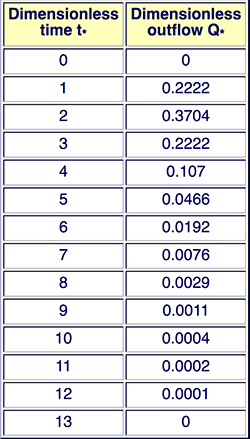
Once the GDUH is chosen, the ordinates of the unit hydrograph may be calculated from Eq. 2-25 as follows:
Likewise, the abscissa (time) may be calculated from Eq. 2-20 as follows:
The unit hydrograph thus calculated may be convoluted with the effective storm hyetograph to determine
the composite flood hydrograph (Ponce, 2014).
The GDUH has the following significant advantages:
The GDUH is solely a function of C and N, and is of global applicability.
Unlike other established unit hydrograph procedures
such as the Natural Resources Conservation Service (NRCS) unit hydrograph, the GDUH is a two-parameter model;
therefore, it is able to simulate a wider range of runoff diffusion effects (Ponce, 2014).
The GDUH cascade parameters (C and N) are estimated based on the runoff diffusion properties of the basin under consideration.
The runoff diffusion properties are largely dependent on the overall terrain's topography and geomorphology. Steep basins have little or no diffusion; conversely, mild basins have substantial amounts of diffusion. The case of zero diffusion is modeled with C = 2 and
In Nature, basins are classified with regards to runoff diffusion on the basis of mean land surface slope. A preliminary classification is shown in
3. METHODOLOGY
3.1 Overview
The methodology for this study
aims to develop a relation between the GDUH cascade parameters C and N
and the respective basin geomorphologic characteristics.
For this purpose, several suitable basins are selected in California, encompassing a broad
range in geomorphologic features, in particular stream channel slope and land surface slope.
For daily data, the time interval of analysis is one day; therefore,
the corresponding duration of the unit hydrograph is 1 day (tr = 1 day).
The selected methodology depends on the temporal storm characteristics.
The following two situations are considered:
Simple storms, featuring a one-day precipitation impulse
(a one-day predominant
precipitation event may be used in practice); and
Complex storms, with a precipitation event
distributed over several days.
3.1.1 Simple storms
For simple storms, the following steps are required:
Assemble the rainfall-runoff data
Assemble corresponding sets of rainfall-runoff data for each watershed/basin, and
identify three (3) suitable infrequent
events for analysis.
Calculate the unit hydrograph runoff volume
Calculate the runoff volume corresponding to 1 cm of effective rainfall.
For each event:
Use the straight line technique of baseflow separation to determine the direct runoff storm hydrograph.
Calculate the runoff volume corresponding to the direct runoff storm hydrograph obtained in Step 3(a), and compare with the runoff volume obtained in Step 2.
Based on the results of Step 3(b), multiply
the direct runoff storm hydrograph ordinates by the appropriate factor
to establish the unit hydrograph ordinates. Confirm that it corresponds to 1 cm of runoff. When warranted,
perform minor volumetric corrections.
Calculate the dimensionless unit hydrograph (DUH) using Eqs. 2-20 and 2-23 for the abscissas and ordinates, respectively.
Calculate the unit hydrograph
Average the three (3) dimensionless unit hydrographs obtained in Step 3 (d) to obtain the watershed/basin's dimensionless
unit hydrograph (DUH).
Confirm that it corresponds to 1 cm of runoff.
Calculate the cascade parameters C and N
Match the dimensionless unit hydrograph peak flow Q*p and
time-to-peak t*p
to a suitable general dimensionless unit hydrograph (GDUH) featuring paired cascade parameters 3.1.2 Complex storms
For complex storms, the follow steps are required:
Assemble the rainfall-runoff data
Assemble corresponding sets of rainfall-runoff data for each watershed/basin,
and identify three (3) suitable infrequent
events for analysis.
For each event:
Use the straight line technique of baseflow separation to determine the direct runoff storm hydrograph.
Calculate the runoff volume corresponding to the direct runoff storm hydrograph.
Apply the φ-index procedure to the total storm hyetograph to determine the effective storm hyetograph (Ponce, 2014a).
Apply the inverse convolution technique to the direct runoff storm hydrograph obtained in Step 2 (b) and the effective storm
hyetograph obtained in Step 2 (c) to calculate the unit hydrograph (Section 3.2).
Calculate the dimensionless unit hydrograph (DUH) using Eqs. 2-20 and 2-23 for the abscissas and ordinates, respectively.
Calculate the unit hydrograph
Average the three (3) dimensionless unit hydrographs obtained in Step 2 (e) to obtain the watershed/basin's unit hydrograph (UH).
Confirm that it corresponds to 1 cm of runoff.
Calculate the cascade parameters C and N
Match the dimensionless unit hydrograph peak flow Q*p and
time-to-peak t*p
to a suitable general dimensionless unit hydrograph (GDUH) featuring paired cascade parameters
For each of the basins analyzed, the set of thus found paired C and N cascade parameters are related to
primary basin geomorphologic characteristics such as channel/land slope.
In a practical application, once the average stream channel slope and land surface slope are determined, the appropriate values of 3.2 Convolution and inverse convolution
Convolution is the procedure by which a certain unit hydrograph and an effective storm hyetograph are used to calculate the
corresponding flood hydrograph. Conversely, inverse convolution is the procedure by which a certain flood hydrograph and an
effective storm hyetograph are used to calculate the corresponding unit hydrograph.
Fig. 3.1 Convolution and inverse convolution.
The convolution procedure is based on the principles of linearity and superposition.
The volume under the composite hydrograph is equal to the total volume of the effective rainfall.
Given Tbu = time base of the X-hour unit hydrograph, and a storm consisting of n X-hour intervals,
the time base of the composite (flood) hydrograph
The convolution procedure is illustrated by the following example. Assume that the following 1-h unit hydrograph has been derived for a certain watershed:
A 6-h storm with a total of 5 cm of effective rainfall covers the entire watershed and is distributed in time as follows:
The composite (flood) hydrograph is calculated using the convolution technique, as follows
The sum of Col. 2 is 2800 m3/s and is equivalent to 1 cm of net rainfall.
The sum of Col. 9 is verified to be 14,000 m3/s, and, therefore, the equivalent of 5 cm of effective rainfall.
The time base of the composite hydrograph is 3.2.2 Inverse convolution The inverse convolution procedure enables the calculation of a unit hydrograph based on an effective storm hyetograph and a composite (flood) hydrograph. The procedure is referred to as method of forward substitution (Ponce, 2014). The unit hydrograph can be calculated directly due to the banded property of the convolution matrix (see Table 3.1). With m = number of nonzero unit hydrograph ordinates, n = number of intervals of effective rainfall, and N = number of nonzero storm hydrograph ordinates, the following relation holds:
Therefore:
By elimination and back substitution, the following formula is developed for the unit hydrograph ordinates ui as a function of storm hydrograph ordinates qi and effective rainfall depths rk , for i varying from 1 to m:
In the summation term of Eq. 3-3, j decreases from j -1 to 1, and k increases from 2 up to a maximum of n. This recursive Eq. 3-3 allows the direct calculation of a unit hydrograph based on a hydrograph from complex storm. In practice, however, it is not always feasible to arrive at a solution because it may be difficult to get a perfect match of composite (flood) hydrograph and effective storm hyetograph (due to noise in the data). Note that the (measured) storm hydrograph would have to be separated into direct runoff and baseflow before attempting to use Eq. 3-3. The inverse convolution procedure is illustrated by applying Eq. 3-3 to the example of Table 3-1. Using Eq. 3-2, with number of nonzero storm hyetograph ordinates N = 13, and number of intervals of effective rainfall n = 6, the number of nonzero unit hydrograph ordinates is: m = 8. Therefore:
This result confirm the ordinates of the unit hydrograph shown in Col. 2 of Table 3-1. 3.3 General dimensionless unit hydrograph
The theory of the general dimensionless unit hydrograph (GDUH) was developed by
Ponce (2009).
An online version of the GDUH as a function of C and N is given in ponce.sdsu.edu/online_general_uh_cascade.
Figure 3.2 shows a sample output for C = 1 and
Fig. 3.2 Dimensionless unit hydrograph for C = 1 and N = 3.
An online version of a GDUH series for a given C (recommended range 0.1 ≤ C ≤ 2.0) and for all N in the range
Fig. 3.3 Dimensionless unit hydrograph for C = 1 and 1 ≤ N ≤ 10.
An online version of a GDUH series for six (6) C values covering the recommended range
(2.0, 1.5, 1.0, 0.5, 0.2, and 0.1), and for all N values in the range 1 ≤ N ≤ 10, is given in
ponce.sdsu.eduonline_all_series_uh_cascade. Figure 3.2 shows a summary table of dimensionless peak discharge Qp* and time of occurrence tp*.
Compare the result for Courant number C = 1 and
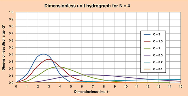
Fig. 3.4 Summary table of dimensionless unit hydrographs for 2 < C ≤ 0.1, and 1 ≤ N ≤ 10. 3.4 Series of dimensionless unit hydrographs Figures 3.5 (a) to (f) show the series of dimensionless unit hydrographs (DUHs) for cascade parameters C with values of 2, 1.5, 1, 0.5, 0.2 and 0.1; and N varying between 1 and 10. The examination of these figures enables the following conclusions:
Fig. 3.5 (a) Dimensionless unit hydrograph for C = 2.
Fig. 3.5 (b) Dimensionless unit hydrograph for C = 1.5.
Fig. 3.5 (c) Dimensionless unit hydrograph for C = 1.
Fig. 3.5 (d) Dimensionless unit hydrograph for C = 0.5.
Fig. 3.5 (e) Dimensionless unit hydrograph for C = 0.2.
Fig. 3.5 (f) Dimensionless unit hydrograph for C = 0.1. Figures 3.6 (a) to (f) show the series of dimensionless unit hydrographs (DUHs) for cascade parameters N with values of 1, 2, 3, 4, 5 and 6; and C varying between 2 and 0.1 as indicated. The examination of these figures enables the following conclusions:
Fig. 3.6 (a) Dimensionless unit hydrograph for N = 1.
Fig. 3.6 (b) Dimensionless unit hydrograph for N = 2.
Fig. 3.6 (c) Dimensionless unit hydrograph for N = 3.
Fig. 3.6 (d) Dimensionless unit hydrograph for N = 4.
Fig. 3.6 (e) Dimensionless unit hydrograph for N = 5.
Fig. 3.6 (f) Dimensionless unit hydrograph for N = 6. 3.5 GDUH, CLR and convolution
The cascade of linear reservoirs (CLR) (Section 2.3) and the convolution of the unit hydrograph with the effective storm hyetograph (Section 3.2.1)
lead to the same composite flood hydrograph, provided
the cascade parameters (GDUH) are used to develop the unit hydrograph for the convolution.
These propositions are substantiated with an example.
Assume the 6-hr effective storm hyetograph shown in Table 3.2.
Assume the basin drainage area: A = 432 km2.
The applicable unit hydrograph duration tr is the same as the
[effective] storm hyetograph time interval (Table 3.2), i.e., tr = Δt = 1 hr.
Assume that the basin has a relatively steep relief, with
cascade parameters C = 1 and N = 2.
An online version of the GDUH as a function of C and N is given in ponce.sdsu.edu/online_general_uh_cascade.
Fig. 3.7 Dimensionless unit hydrograph for C = 1 and N = 2. Given the reservoir storage constant K:
and time
and discharge
the program ponce.sdsu.edu/online_dimensionless_uh_cascade
gives the unit hydrograph and dimensionless unit hydrograph shown in Fig. 3.8.
Fig. 3.8 Unit hydrograph and dimensionless unit hydrograph for C = 1 and N = 2.
With C = 1 (i.e., K = 1), N = 2, and the given effective storm hyetograph (Table 3.2), the program
ponce.sdsu.edu/online_routing_08
calculates the composite flood hydrograph by the cascade of linear
reservoirs (Ponce 1989).
The composite flood hydrograph is shown in Fig. 3.9.
Fig. 3.9 Composite flood hydrograph by the cascade of linear reservoirs (CLR).
The convolution of the unit hydrograph (Fig. 3.8, Cols. 2 and 3) with the effective storm hyetograph (Table 3.2) is accomplished using the program
ponce.sdsu.edu/online_convolution.
For this example, an effective storm hyetograph is applicable;
therefore, the curve number is: CN = 100.
The composite flood hydrograph is shown in Fig. 3.10. Remarkably, it is confirmed that the results of
Fig. 3.10 Composite flood hydrograph by convolution.
In summary, given a set of cascade parameters C and N, and an effective storm hyetograph, the method of cascade of linear reservoirs (CLR) can be used to
calculate a composite flood hydrograph.
Likewise, the convolution of a unit hydrograph derived with the GDUH method,
using the same set of cascade parameters (C and N),
can be used to calculate a composite flood hydrograph.
It is shown that
these two flood hydrographs are the same.
4. DATA ANALYSIS
4.1 Rationale Several basins in California are selected, with wide ranging geomorphological features. The basins meet the following requirements:
4.2 Data sources The hydrometeorological and geomorphological data was collected from the following sources:
4.3 Geomorphological parameters 4.3.1 Drainage area The drainage area determines the potential runoff volume, provided the storm covers the whole area. The catchment divide is the loci of points delimiting two adjacent catchments, i.e., the collection of high points (peaks and saddles) separating catchments draining into different outlets. In this study, catchment areas were obtained with the aid of GIS. 4.3.2 Drainage perimeter The perimeter of the drainage area is the sum of the length delineating the catchment. Catchment perimeters were obtained with the aid of GIS. 4.3.3 Catchment hydraulic length The hydraulic length is the length measured along the principal watercourse. The principal watercourse (or main stream) is the central and largest watercourse of the catchment and the one conveying the flow to the outlet. Hydraulic lengths were obtained with the aid of GIS. 4.3.4 Form ratio The form ratio is defined as follows:
in which Kf = form ratio, A = catchment area, and L = catchment length, measured along the longest watercourse. Area and length are given in consistent units such as square kilometers and kilometers, respectively. 4.3.5 Compactness ratio An alternate morphological description is based on catchment perimeter rather than area. For this purpose, an equivalent circle is defined as a circle of area equal to that of the catchment. The compactness ratio is the ratio of the catchment perimeter to that of the equivalent circle. This leads to:
in which Kc = compactness ratio, P = catchment perimeter, and A = catchment area, with P and A given in any consistent set of units. 4.3.6 Maximum and minimum elevation The maximum elevation is the highest point in the catchment divide, while the minimum elevation is the catchment outlet. The difference between these two reference points is the catchment relief. Catchment elevations were obtained with the aid of GIS. 4.3.7 Average land surface slope Grid methods are often used to obtain measures of land surface slope for runoff evaluations. For instance, the USDA Natural Resources Conservation Service (NRCS) determines average surface slope by overlaying a square grid pattern over the topographic map of the watershed. The maximum surface slope at each grid intersection is evaluated, and the average of all values calculated. This average is taken as the representative value of land surface slope. The procedure was performed with the aid of GIS, and the average land surface slope referred to as S0. 4.3.8 Stream channel slope The channel gradient of a principal watercourse is a convenient indicator of catchment relief. A longitudinal profile is defined by its maximum (upstream) and minimum (downstream) elevations, and by the horizontal distance between them. The channel gradient obtained directly from the upstream and downstream elevations is referred to as the S1 slope. An alternate stream channel slope is obtained by calculating the slope between two points in the profile, located at 10% and 85% from the mouth, respectively. This procedure is recommended by the U.S. Geological Survey (Ponce, 2014a). This stream channel slope is referred to as S2. 4.3.9 Total stream channel length The total stream channel length is the sum of all stream channels defined inside the cachtment. This procedure was performed with the aid of GIS. 4.3.10 Drainage density The catchment's drainage density is the ratio of total stream length to catchment area. A high drainage density reflects a fast and peaked runoff response, whereas a low drainage density is characteristic of a delayed runoff response. 4.3.11 Mean annual precipitation Rainfall varies not only temporally but also spatially, i.e., the same amount of rain does not fall uniformly over the entire catchment. Isohyets are used to depict the spatial variation of rainfall. An isohyet is a contour line showing the loci of equal rainfall depth. Isohyetal analysis was performed with the aid of GIS. 4.4 Selection of basins Ten (10) basins located in California were selected for analysis. The basins are listed in Table 4.1.
4.4.1 Campo Creek near Campo, CA The headwaters of Campo Creek are located near the community of Live Oak Springs, in southeast San Diego County, California (Fig. 4.1). The stream flows in a predominantly southwestern direction toward the community of Campo (Fig. 4.2). The National Weather Service (NWS) meteorological station is located in Campo (Fig. 4.3). The USGS streamgaging station is located at the intersection of Campo Creek with California State Route 94 (Fig. 4.4).
Fig. 4.1 Downstream view of Campo Creek near its headwaters.
Fig. 4.2 Upstream view of Campo Creek in Campo valley, California.
Fig. 4.3 NOAA NWS raingage at Campo, California.
Fig. 4.4 USGS streamgaging station at the intersection of Campo Creek with SR 94.
After crossing into Mexico, Campo Creek is renamed Cañada Joe Bill, which flows into Tecate Creek at Tecate. In turn, Tecate Creek flows into the Tijuana River, the latter eventually discharging into the Pacific Ocean at Imperial Beach, California.
Fig. 4.5 Aerial view of the Campo Creek subbasin.
Fig. 4.6 Hydrologic map of the Campo Creek subbasin.
Figure 4.7 shows the three (3) flood hydrographs selected for analysis.
Fig. 4.7 (a) Campo Creek near Campo, California: Flood hydrograph No. 1 - Year 1983.
Fig. 4.7 (b) Campo Creek near Campo, California: Flood hydrograph No. 2 - Year 1993.
Fig. 4.7 (c) Campo Creek near Campo, California: Flood hydrograph No. 3 - Year 1998.
The headwaters of Whitewater river at located near San Gorgonio Mountain, in southeast Forest Falls, California. The stream flows in a predominantly southeastern direction toward the community of Whitewater (Fig. 4.8), flowing into the Salton Sea (Fig. 4.9). The National Weather Service (NWS) meteorological stations are located in Palm Springs, Palm Desert and Indio. The USGS streamgaging station is located near its mouth at the Salton Sea.
Fig. 4.8 The Whitewater river canyon.
Fig. 4.9 Mouth of the Whitewater river at the Salton Sea.
Figure 4.10 shows the outline of the Whitewater river basin. Most of the basin is located in Riverside County; however, a very small fraction is located in San Bernardino County. This basin has been one of southern California's most important agricultural regions, which corresponds to Koppen's winter/hot summer climate. The mean annual precipitation is 112 mm (4.41 in). Figures 4.11 and 4.12 show the hydrologic map and the mean annual precipitation map of the Whitewater river basin.
Fig. 4.10 Aerial view of the Whitewater river basin.
Fig. 4.11 Hydrologic map of the Whitewater river basin.
Fig. 4.12 Mean annual precipitation map of the Whitewater river basin.
Table 4.4 shows precipitation and streamgaging data sources from the Whitewater river basin.
Figure 4.13 shows the three (3) flood hydrographs selected for analysis.
Fig. 4.13 (a) Whitewater river near Mecca, California: Flood hydrograph No. 1 - Year 2008.
Fig. 4.13 (b) Whitewater river near Mecca, California: Flood hydrograph No. 2 - Year 2008.
Fig. 4.13 (c) Whitewater river near Mecca, California: Flood hydrograph No. 3 - Year 2015. The headwaters of the Mojave river are located near the highlands of Indian Wells, Cantil, Peasonville, Darwin, Afton Canyon (Fig. 4.14), Blanco Mountain, Sylvana Mountain, Gold Mountain, Palmer Mountain, Beatty, Amargosa Valley, Clark Mountain and Baker. The stream flows in a predominantly southern direction toward the community of Helendale (Fig. 4.15). The National Weather Service (NWS) meteorological stations are located in Pearblossom, Palmdale, Lancaster, Mojave, Barstow, Randsburg, China Lake, Trona and Stovepipe wells. The USGS streamgaging station is located at the intersection of National Trails Highway with Mojave Heights.
Fig. 4.14 The Mojave river at Afton Canyon, California.
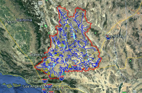
Fig. 4.15 The Mojave river at Helendale, California. Figure 4.16 shows the outline of the Mojave river basin. The basin is located in Kern, Los Angeles, San Bernardino and Inyo Counties of California; and Goldfiel, Beatty, Yucca Flat, Amargosa Valley and Pahrump Counties of Nevada. The weather corresponds to Koppen's desert climate (BWk). The mean annual precipitation is 109 mm (4.29 in). Figures 4.17 and 4.18 show the hydrologic map and the mean annual precipitation map of the Mojave river basin.
Fig. 4.16 Aerial view of the Mojave river basin.
Fig. 4.17 Hydrologic map of the Mojave river basin.
Fig. 4.18 Mean annual precipitation map of the Mojave river basin.
Table 4.6 shows precipitation and streamgaging data sources from the Mojave river basin.
Figure 4.19 shows the three (3) flood hydrographs selected for analysis.
Fig. 4.19 (a) Mojave river near Victorville, California: Flood hydrograph No. 1 - Year 2010.
Fig. 4.19 (b) Mojave river near Victorville, California: Flood hydrograph No. 2 - Year 2017.
Fig. 4.19 (c) Mojave river near Victorville, California: Flood hydrograph No. 3 - Year 2017. The headwaters of the Amargosa river at located near Beatty, Timber Mountain, Black Mountain, Shoshone and Amargosa Valley (Fig. 4.20). The stream flows in a predominantly southeastern direction toward the communities of Beatty, Amargosa Valley, Evelyn, Shoshone and Tecopa (Fig. 4.21). The National Weather Service (NWS) meteorological station is located in Shoshone. The USGS streamgaging station is located near Tecopa, California.
Fig. 4.20 Upstream view of Amargosa river.
Fig. 4.21 View of Amargosa river near Shoshone, California. Figure 4.22 shows the outline of the Amargosa river basin. The basin is located in Inyo County of California; and Beatty, Yucca Flat, Amargosa Valley and Pahrump Counties of Nevada. The weather corresponds to Koppen's cold desert climate (BWk). The mean annual precipitation is 110 mm (4.32 in). Figures 4.23 and 4.24 show the hydrologic map and the mean annual precipitation map of the Amargosa river basin.
Fig. 4.22 Aerial view of the Amargosa river basin.
Fig. 4.23 Hydrologic map of the Amargosa river basin.
Table 4.8 shows precipitation and streamgaging data sources from the Amargosa river basin.
Figure 4.24 shows the three (3) flood hydrographs selected for analysis.
Fig. 4.24 (a) Amargosa river near Tecopa, California: Flood hydrograph No. 1 - Year 2007.
Fig. 4.24 (b) Amargosa river near Tecopa, California: Flood hydrograph No. 2 - Year 2008.
Fig. 4.24 (c) Amargosa river near Tecopa, California: Flood hydrograph No. 3 - Year 2010. 4.4.5 Petaluma river near Petaluma, CA The headwaters of the Petaluma river at located near Sonoma Mountain. The stream flows in a predominantly southweastern direction toward the communities of Penngrove and Petaluma (Fig. 4.25). The National Weather Service (NWS) meteorological station is located in Petaluma (Fig. 4.26). The USGS streamgaging station is located near Petaluma, California.
Fig. 4.25 The Petaluma river at Petaluma, California.
Fig. 4.26 The Petaluma river at the USGS streamgaging station.
Figure 4.27 shows the outline of the Petaluma river basin. The basin is located in Sonoma County of California. The weather corresponds to Koppen's mild Mediterranean climate. The mean annual precipitation is 624 mm (24.57 in). Figure 4.28 shows the hydrologic map of the Petaluma River basin.
Fig. 4.27 Aerial view of the Petaluma river basin.
Fig. 4.28 Hydrologic map of the Petaluma river basin.
Table 4.10 shows precipitation and streamgaging data sources from the Petaluma river Basin.
Figure 4.29 shows the three (3) flood hydrographs selected for analysis.
Fig. 4.29 (a) Petaluma river near Petaluma, California: Flood hydrograph No. 1 - Year 2000.
Fig. 4.29 (b) Petaluma river near Petaluma, California: Flood hydrograph No. 2 - Year 2002.
Fig. 4.29 (c) Petaluma river near Petaluma, California: Flood hydrograph No. 3 - Year 2010. 4.4.6 Russian river near Guerneville, CA The headwaters of the Russian river at located near Saint Helena Mountain, Red Mountain, and the highlands of Potter and Redwood valleys. The stream flows in a predominantly southeastern direction toward the communities of Potter Valley, Redwood Valley, Ukiah, El Roble, Largo, Hopland, Pieta, Preston, Cloverdale, Asti, Geyserville (Fig. 4.30), Healdsburg and Guerneville (Fig. 4.31). The National Weather Service (NWS) meteorological stations are located in Potter Valley, Ukiah and Cloverdale. The USGS streamgaging station is located near Guerneville.
Fig. 4.30 The Russian river at Gerseyville, California.
Fig. 4.31 The Russian river at Guerneville, California.
Figure 4.32 shows the outline of the Russian river basin. The basin is located in Mendocino and Sonoma Counties in California. The weather corresponds to Koppen's hot-summer Mediterranean climate (Csa). The mean annual precipitation is 1072 mm (42.20 in). Figures 4.33 and 4.34 show the hydrologic map and the mean annual precipitation map of the Russian river basin.
Fig. 4.32 Aerial view of the Russian river basin.
Fig. 4.33 Hydrologic map of the Russian river basin.
Fig. 4.34 Mean annual precipitation map of the Russian river basin.
Table 4.12 shows precipitation and streamgaging data sources from the Russian River basin.
Figure 4.35 shows the three (3) flood hydrographs selected for analysis.
Fig. 4.35 (a) Russian river near Guerneville, California: Flood hydrograph No. 1 - Year 1994.
Fig. 4.35 (b) Russian river near Guerneville, California: Flood hydrograph No. 2 - Year 1995.
Fig. 4.35 (c) Russian river near Guerneville, California: Flood hydrograph No. 3 - Year 1998. 4.4.7 Los Gatos Creek near Coalinga, CA The headwaters of Los Gatos Creek at located near Santa Rita and Condon Peak. The stream flows in a predominantly southeastern direction toward the community of Coalinga (Fig. 4.36). The National Weather Service (NWS) meteorological station is located in Coalinga. The USGS streamgaging station is located upstream at Coalinga (Fig. 4.37).
Fig. 4.36 Los Gatos Creek near Coalinga, California.
Fig. 4.37 Los Gatos Creek upstream of Coalinga, California.
Figure 4.38 shows the outline of Los Gatos Creek basin. The basin is located in Fresno County in California. The weather corresponds to Koppen's cold/summer Mediterranean climate. The mean annual precipitation is 394 mm (15.51 in). Figure 4.39 shows the hydrologic map of Los Gatos Creek basin.
Fig. 4.38 Aerial view of Los Gatos Creek basin.
Fig. 4.39 Hydrologic map of Los Gatos Creek basin.
Table 4.14 shows precipitation and streamgaging data sources from Los Gatos Creek basin.
Figure 4.40 shows the three (3) flood hydrographs selected for analysis.
Fig. 4.40 (a) Los Gatos Creek near Coalinga, California: Flood hydrograph No. 1 - Year 1977.
Fig. 4.40 (b) Los Gatos Creek near Coalinga, California: Flood hydrograph No. 2 - Year 1978.
Fig. 4.40 (c) Los Gatos Creek near Coalinga, California: Flood hydrograph No. 3 - Year 1978. 4.4.8 Cottonwood Creek near Cottonwood, CA The headwaters of Cottonwood Creek at located near Lazyman Butte, North Yolla Bolly and highlands of Platina. The stream flows in a predominantly northeastern direction toward the communities of Platina, Ono and Cottonwood (Fig. 4.41). The National Weather Service (NWS) meteorological station is located in the highlands of Platina. The USGS streamgagin station is located near Cottonwood.
Fig. 4.41 Cottonwood Creek at Cottonwood, California.
Figure 4.42 shows the outline of Cottonwood Creek basin. The basin is located in Shasta and Tehama Counties in California. The weather corresponds to Koppen's warm-summer Mediterranean climate (Csa). The mean annual precipitation is 876 mm (34.49 in). Figure 4.43 shows the hydrologic map of the Cottonwood Creek basin.
Fig. 4.42 Aerial view of Cottonwood Creek basin.
Fig. 4.43 Hydrologic map of Cottonwood Creek basin.
Table 4.16 shows precipitation and streamgaging data sources from the Cottonwood Creek basin.
Figure 4.44 shows the three (3) flood hydrographs selected for analysis.
Fig. 4.44 (a) Cottonwood Creek near Cottonwood, California: Flood hydrograph No. 1 - Year 1993.
Fig. 4.44 (b) Cottonwood Creek near Cottonwood, California: Flood hydrograph No. 2 - Year 1996.
Fig. 4.44 (c) Cottonwood Creek near Cottonwood, California: Flood hydrograph No. 3 - Year 1998. 4.4.9 Salinas river near Spreckels, CA The headwaters of the Salinas river at located near Machesna Mountain, Tassajera Peak; and the hihglands of Atascadero, Paso Robles, King City, Greenfield and Salinas. The stream flows in a predominantly northwestern direction toward the communities of San Ardo (Fig. 4.45), Shandon, Atascadero, Paso Robles (Fig. 4.46), San Miguel, Bradley, San Lucas, King City, Greenfield, Soledad, Gonzales, Chualar and Salinas. The National Weather Service (NWS) meteorological stations are located in Santa Margarita, Paso Robles and King City. The USGS streamgaging station is located near Spreckels, California.
Fig. 4.45 Salinas river at San Ardo, California.
Fig. 4.46 Salinas river at Paso Robles, California.
Figure 4.47 shows the outline of the Salinas river basin. The basin is located in San Luis Obispo, San Benito and Monterey Counties in California. The weather corresponds to Koppen's semi-arid and dry steppe and Mediterranean climate (Csb). The mean annual precipitation is 294 mm (11.57 in). Figures 4.48 and 4.49 show the hydrologic map and the mean annual precipitation map of the Salinas river basin.
Fig. 4.47 Aerial view of Salinas river basin.
Fig. 4.48 Hydrologic map of Salinas river basin.
Fig. 4.49 Mean annual precipitation map of Salinas river basin.
Table 4.18 shows precipitation and streamgaging data sources from the Salinas river basin.
Figure 4.50 shows the three (3) flood hydrographs selected for analysis.
Fig. 4.50 (a) Salinas river near Spreckels, California: Flood hydrograph No. 1 - Year 1980.
Fig. 4.50 (b) Salinas river near Spreckels, California: Flood hydrograph No. 2 - Year 1983.
Fig. 4.50 (c) Salinas river near Spreckels, California: Flood hydrograph No. 3 - Year 1995. 4.4.10 Shasta river near Montague, CA The headwaters of the Shasta river at located near Mount Shasta and China Mountain. The stream flows in a predominantly northwestern direction toward Edgewood (Fig. 4.51), Gazelle, Grenada and Montague (Fig. 4.52). The National Weather Service (NWS) meteorological station is located in Weed. The USGS streamgaging station is located near Montague, California.
Fig. 4.51 Shasta river at Edgewood, California.
Fig. 4.52 Shasta river at Montague, California.
Figure 4.53 shows the outline of Shasta river basin. The basin is located in Siskiyou County in California. The weather corresponds to Koppen's warm-summer Mediterranean climate. The mean annual precipitation is 478 mm (18.82 in). Figure 4.54 shows the hydrologic map of the Shasta river basin.
Fig. 4.53 Aerial view of Shasta river basin.
Fig. 4.54 Hydrologic map of Shasta river basin.
Table 4.20 shows precipitation and streamgaging data sources from the Shasta river basin.
Figure 4.55 shows the three (3) flood hydrographs selected for analysis.
Fig. 4.55 (a) Shasta river near Montague, California: Flood hydrograph No. 1 - Year 2002.
Fig. 4.55 (b) Shasta river near Montague, California: Flood hydrograph No. 2 - Year 2005.
Fig. 4.55 (c) Shasta river near Montague, California: Flood hydrograph No. 3 - Year 2015.
5. GDUH MODEL APPLICATION
5.1 Data analysis Following Section 3, the data analysis may be based on: (a) simple storms, or (b) complex storms. For the most part, the inherent noisiness of the data precluded application using complex storms. Accordingly, simple storms were chosen for general application as a practical compromise. Three (3) corresponding event sets of rainfall-runoff data were assembled for each basin. Example results corresponding to Campo Creek are summarized in Tables 5.1 and 5.2. Table 5.1 shows the following:
Table 5.2 shows the following:
5.1.1 Campo Creek
Following the procedure described in Section 3.1.1, three (3) corresponding event sets of rainfall-runoff data were assembled for Campo Creek.
The results are summarized in Tables 5.3 and 5.4.
Figure 5.1 shows average measured vs predicted dimensionless unit hydrographs (DUH) for the Campo Creek subbasin, obtained by plotting Col. 1 vs Cols. 5 and 6 of Table 5.4, respectively.
Fig. 5.1 Campo Creek subbasin: Average measured vs predicted DUH. 5.1.2 Whitewater River
Following the procedure described in Section 3.1.2, three (3) corresponding event sets of rainfall-runoff data were assembled for Whitewater river.
The results are summarized in Tables
Figure 5.2 shows average measured vs predicted dimensionless unit hydrographs (DUH) for the Whitewater river basin, obtained by plotting Col. 1 vs Cols. 5 and 6 of Table 5.6, respectively.
Fig. 5.2 Whitewater river basin: Average measured vs predicted DUH. 5.1.3 Mojave River
Following the procedure described in Section 3.1.3, three (3) corresponding event sets of rainfall-runoff data were assembled for Mojave river.
The results are summarized in Tables
Figure 5.3 shows average measured vs predicted dimensionless unit hydrographs (DUH) for the Mojave river basin, obtained by plotting Col. 1 vs Cols. 5 and 6 of Table 5.8, respectively.
Fig. 5.3 Mojave river basin: Average measured vs predicted DUH. 5.1.4 Amargosa River
Following the procedure described in Section 3.1.4, three (3) corresponding event sets of rainfall-runoff data were assembled for Amargosa river.
The results are summarized in Tables
Figure 5.4 shows average measured vs predicted dimensionless unit hydrographs (DUH) for the Amargosa river basin, obtained by plotting Col. 1 vs Cols. 5 and 6 of Table 5.10, respectively.
Fig. 5.4 Amargosa river basin: Average measured vs predicted DUH. 5.1.5 Petaluma River
Following the procedure described in Section 3.1.5, three (3) corresponding event sets of rainfall-runoff data were assembled for Petaluma river.
The results are summarized in Tables
Figure 5.5 shows average measured vs predicted dimensionless unit hydrographs (DUH) for the Petaluma river basin, obtained by plotting Col. 1 vs Cols. 5 and 6 of Table 5.12, respectively.
Fig. 5.5 Petaluma river basin: Average measured vs predicted DUH. 5.1.6 Russian River
Following the procedure described in Section 3.1.6, three (3) corresponding event sets of rainfall-runoff data were assembled for Petaluma river.
The results are summarized in Tables
Figure 5.6 shows average measured vs predicted dimensionless unit hydrographs (DUH) for the Russian river basin, obtained by plotting Col. 1 vs Cols. 5 and 6 of Table 5.14, respectively.
Fig. 5.6 Russian river basin: Average measured vs predicted DUH. 5.1.7 Los Gatos Creek
Following the procedure described in Section 3.1.7, three (3) corresponding event sets of rainfall-runoff data were assembled for Los Gatos Creek.
The results are summarized in Tables
Figure 5.7 shows average measured vs predicted dimensionless unit hydrographs (DUH) for the Los Gatos creek basin, obtained by plotting Col. 1 vs Cols. 5 and 6 of Table 5.16, respectively.
Fig. 5.7 Los Gatos creek basin: Average measured vs predicted DUH. 5.1.8 Cottonwood Creek
Following the procedure described in Section 3.1.8, three (3) corresponding event sets of rainfall-runoff data were assembled for Cottonwood Creek.
The results are summarized in Tables
Figure 5.8 shows average measured vs predicted dimensionless unit hydrographs (DUH) for the Cottonwood creek basin, obtained by plotting Col. 1 vs Cols. 5 and 6 of Table 5.18, respectively.
Fig. 5.8 Cottonwood creek basin: Average measured vs predicted DUH. 5.1.9 Salinas River
Following the procedure described in Section 3.1.9, three (3) corresponding event sets of rainfall-runoff data were assembled for Salinas river.
The results are summarized in Tables
Figure 5.9 shows average measured vs predicted dimensionless unit hydrographs (DUH) for the Salinas river basin, obtained by plotting Col. 1 vs Cols. 5 and 6 of Table 5.20, respectively.
Fig. 5.9 Salinas river basin: Average measured vs predicted DUH. 5.1.10 Shasta River
Following the procedure described in Section 3.1.10, three (3) corresponding event sets of rainfall-runoff data were assembled for Shasta river.
The results are summarized in Tables
Figure 5.10 shows average measured vs predicted dimensionless unit hydrographs (DUH) for the Shasta river basin, obtained by plotting Col. 1 vs Cols. 5 and 6 of Table 5.22, respectively.
Fig. 5.10 Shasta river basin: Average measured vs predicted DUH. 5.2 Analysis of results
For illustration purposes, Fig. 5.7 is repeated here. It is shown that all ten (10) cases studied
Fig. 5.7 Los Gatos Creek basin: Average measured vs predicted DUH. 5.3 Geomorphological analysis
In this section, measured geomorphological parameters described in Section 4.3 are related to predicted CLR parameters described
in Section 5.1.
Figure 5.11 shows the calculated C/N pairs for the indicated basins. In general, a lower value of
Fig. 5.11 C/N pairs for indicated basins.
Figure 5.12 shows the relation between DUH peak discharge Qp* and time-to-peak
tp* for the ten (10) basins studied. This graph shows an increase
in hydrograph diffusion with a decrease in stream channel slope (compare No. 7 and No. 9).
Fig. 5.12 Qp* vs tp* for indicated basins. 5.4 Modeling of unit hydrograph diffusion
Section 3.4 shows that hydrograph diffusion increases with an increase in the value of N and a decrease in the value of C. Accordingly, a diffusion number D may be defined as follows:
Figures 5.13 to 5.16 show the correlation of the diffusion number D with pertinent geomorphological parameters:
(1) drainage basin area A, (2) average land surface slope S0, (3) stream channel slope
S1, and (4) stream channel slope S2 (refer to Table 5.23). The results of these
correlations are summarized in Table 5.24.
Fig. 5.13 Diffusion number D vs drainage basin area A.
Fig. 5.14 Diffusion number D vs average land surface slope S0.
Fig. 5.15 Diffusion number D vs stream channel slope S1.
Fig. 5.16 Diffusion number D vs stream channel slope S2.
Table 5.24 shows that diffusion number D correlates reasonably well with drainage basin area A, and to a lesser extent with stream channel slope S1. In a practical application, given a value of A or S1, the correlations show in this table may be used to calculate D.
Figures 5.17 and 5.18 show the correlation of the number of linear reservoirs N with the following geomorphological
parameters: (1) drainage basin area A, and (2) stream channel slope S1. Given the value of A
or S1, the correlation shown in these figures may be used to calculate N.
Fig. 5.17 Number of linear reservoirs N vs drainage basin area A.
Fig. 5.18 Number of linear reservoirs N vs stream channel slope S1.
6. SUMMARY AND CONCLUSIONS
6.1 Summary The present study validates the theory of the general dimensionless unit hydrograph (GDUH) using California watershed/basin data. The GDUH is a dimensionless formulation of the concept of unit hydrograph, of general applicability and of global scope. Given a basin of drainage area A, for which a unit hydrograph of duration tr is sought, the GDUH methodology provides a dimensionless unit hydrograph (DUH) which is solely based on the cascade of linear reservoirs (CLR) parameters C and N, wherein C = Courant number and N = number of linear reservoirs. The methodology is based on matching an average measured DUH with a predicted DUH. Ten (10) suitable basins were selected in California, covering a broad range of geomorphological parameters, including drainage area, average land surface slope, and stream channel slope. Rainfall-runoff data was analyzed for each basin. Three (3) infrequent flood events were chosen, leading to three (3) unit hydrographs, from which an average measured DUH was obtained. Using the CLR model, a predicted DUH, with parameters C and N, was calculated by trial and error to match the average measured DUH.
A diffusion parameter D was defined to assist in the appropriate modeling of unit hydrograph diffusion. Since the latter increases
with an increase in N and a decrease in C, a first approximation for D was taken as: The methodology developed in this study provides a way to link the shape of the unit hydrograph, i.e., the amount of runoff diffusion, to the geomorphological characteristics of the watershed/basin. It is noted that this objective has been at the center of unit hydrograph research for many decades. Additional applications across the globe ought to provide more information to strengthen the correlations beyond this first attempt at validation of the GDUH theory. 6.2 Conclusions The following conclusions are derived from this study:
6.3 Recommendations The following recomendations are offered for future work:
REFERENCES
Dooge, J. C. I. (1973). Linear theory of hydrologic systems. Technical Bulletin No. 1468, Agricultural Research Service, U.S. Department of Agriculture, Washington, D.C. http://ponce.sdsu.edu/lineartheo232.html
Dooge, J. C. I., W. B. Strupczewski, and J. J. Napiorkowski (1982). Hydrodynamic derivation of storage parameters of the Muskingum model. Journal of Hydrology, Vol. 54, 371-387. http://ponce.sdsu.edu//dooge_hydrodynamic_derivation_1982.pdf
Hayami, S. (1951). On the propagation of flood waves. Bulletin No. 1, Disaster Prevention Research Institute, Kyoto University, Kyoto, Japan, December. http://ponce.sdsu.edu/milestone_hayami_first_page.html
Hoyt, W. G. et. al. (1936). Studies of relations of rainfall and runoff in the United States, Lighthill, M. J., and Whitham, G. B.(1955). On kinematic waves: I. Flood movement in long rivers. Proceedings, Royal Society of London, Series A, 229, 281-316. http://ponce.sdsu.edu/lighthillandwhitham281.html
Linsley, R. K., M. A. Kohler, and L. H. Paulhus. (1962). Hydrology for Engineers, Third edition, McGraw-Hill, New York.
Nash, J. E. (1957). The form of the instantaneous unit hydrograph, Ponce, V. M., and D. B. Simons (1977). Shallow wave propagation in open channel flow. Ponce, V. M. (1980). Linear reservoirs and numerical diffusion. Journal of the Hydraulics Division, Proceedings of the American Society of Civil Engineers, Vol. 106, No. HY5, 691-699. Ponce, V. M. (1989). Engineering hydrology, principles and practices, Prentice Hall, Englewood Cliffs, New Jersey. http://ponce.sdsu.edu/textbook_hydrology_chapters.html
Ponce, V. M. (1991a). The kinematic wave controversy. Journal of Hydraulic Engineering, ASCE, Vol. 117, No. 4, 511-525, April. http://ponce.sdsu.edu/the_kinematic_wave_controversy.html
Ponce, V. M. (1991b). New perspective on the Vedernikov number. Water Resources Research, Vol. 27, No. 7, 1777-1779, July. http://ponce.sdsu.edu/new_perspective_on_the_vedernikov_number.html
Ponce, V. M., O. I. Cordero-Braña, and S. Y. Hasenin (1997). Generalized conceptual modeling of dimensionless overland flow hydrographs. Journal of Hydrology, 200, 222-227. http://ponce.sdsu.edu/generalized_conceptual_modeling_of_dimensionless_overland_flow_hydrographs.html
Ponce, V. M., and A. C. Klabunde (1999). Parking lot storage modeling using diffusion waves. Journal of Hydrologic Engineering, Vol. 4, No. 4, October, 371-376. http://ponce.sdsu.edu/parkinglot371view.html
Ponce, V. M. (2009a). A general dimensionless unit hydrograph. Online report.
Ponce, V. M. (2009b). Cascade and convolution: One and the same. Online report.
http://ponce.sdsu.edu//cascade_and_convolution.html
Ponce, V. M. (2014a). Engineering hydrology, principles and practices, Second Edition, Online.
http://ponce.sdsu.edu/enghydro/
Ponce, V. M. (2014b). Runoff diffusion reexamined. Online report.
http://ponce.sdsu.edu/runoff_diffusion_reexamined.html
Sherman, L. K. (1932). Streamflow from rainfall by unit-graph method, Rodríguez-Iturbe, I. and Valdés, J. B. (1979). The geomorphologic structure of hydrologic response. Water Resources Research, Vol. 15, No. 6, 1409-1420. Rodríguez-Iturbe, I.; Devoto, G. and Valdés, J. B. (1979). Discharge response analysis and hydrologic similarity: the interrelation between the geomorphologic IUH and the storms characteristics. Water Resources Research, Vol. 15, No. 6, 1435-1444. U.S. Army Engineer North Pacific Division. (1972). Program Description and User Manual for SSARR Model, Streamflow Synthesis and Reservoir Regulation, revised June 1975, Portland, Oregon.
Valdés, J. B., Fiallo, Y. and Rodríguez-Iturbe, I. (1979). A rainfall-runoff analysis of the geomorphologic IUH. Water Resources Research, Vol. 15, No. 6, 1421-1434.
|
|||||||||||||||||||||||||||||||||||||||||||||||||||||||||||||||||||||||||||||||||||||||||||||||||||||||||||||||||||||||||||||||||||||||||||||||||||||||||||||||||||||||||||||||||||||||||||||||||||||||||||||||||||||||||||||||||||||||||||||||||||||||||||||||||||||||||||||||||||||||||||||||||||||||||||||||||||||||||||||||||||||||||||||||||||||||||||||||||||||||||||||||||||||||||||||||||||||||||||||||||||||||||||||||||||||||||||||||||||||||||||||||||||||||||||||||||||||||||||||||||||||||||||||||||||||||||||||||||||||||||||||||||||||||||||||||||||||||||||||||||||||||||||||||||||||||||||||||||||||||||||||||||||||||||||||||||||||||||||||||||||||||||||||||||||||||||||||||||||||||||||||||||||||||||||||||||||||||||||||||||||||||||||||||||||||||||||||||||||||||||||||||||||||||||||||||||||||||||||||||||||||||||||||||||||||||||||||||||||||||||||||||||||||||||||||||||||||||||||||||||||||||||||||||||||||||||||||||||||||||||||||||||||||||||||||||||||||||||||||||||||||||||||||||||||||||||||||||||||||||