CHAPTER 7:
STEADY GRADUALLY VARIED FLOW |
7.1 EQUATION OF GRADUALLY VARIED FLOW
The flow is gradually varied when the discharge Q is constant but the other
hydraulic variables (A, V, D, R, P, and so on) vary gradually in space.
The basic assumptions of gradually varied flow are:
The flow is steady, i.e., none of the hydraulic variables vary in time.
The streamlines are essentially parallel; thus,
the pressure distribution in the vertical direction is hydrostatic, i.e., proportional to the flow depth.
The head loss is the same as that corresponding to uniform flow; therefore, the uniform
flow formula may be used to evaluate the energy slope.
The value of Manning's n is the same as that of uniform flow.
Other assumptions of gradually varied flow are:
The slope of the channel is small.
The pressure correction factor cosθ ≅ 1.
There is negligible air entrainment.
The conveyance is an exponential function of the flow depth (except for the case of circular culverts).
The roughness (Manning's n) is independent of the flow depth (only an approximation) and is constant
throughout the reach under consideration.
|
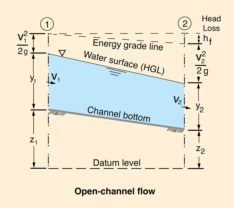
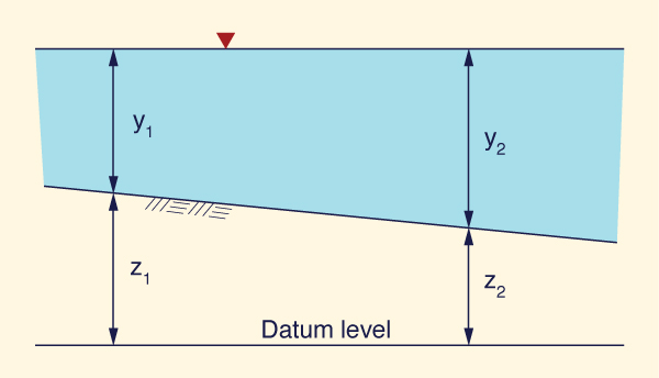
Fig. 7-1 Definition sketch for energy in open-channel flow.
|
|
Under gradually varied flow, the gradient of hydraulic head is (Fig. 7-1):
dH d V 2
_____ = ___ ( z + y + _____ ) = - Sf
dx dx 2g
| (7-1) |
The negative sign in front of the friction slope Sf is required because the flow direction is from left to right,
while the derivative is taken from right to left, by convention. By definition, the friction slope is:
in which ΔL = length of the channel reach under consideration. The gradient of specific energy is:
dE d V 2 dz
_____ = ___ ( y + _____ ) = - ____ - Sf
dx dx 2g dx
| (7-3) |
The gradient of the channel bed, or channel slope (bottom slope), is:
dz z2 - z1
_____ = ________
dx ΔL
| (7-4) |
dz z1 - z2
- _____ = ________ = So
dx ΔL
| (7-5) |
Therefore, the gradient of specific energy is:
dE d V 2
_____ = ___ ( y + _____ ) = So - Sf
dx dx 2g
| (7-6) |
Under steady flow: Q = V A = constant. Therefore:
d Q 2
____ ( y + _______ ) = So - Sf
dx 2g A2
| (7-7) |
dy d Q 2
_____ + _____ ( _______ ) = So - Sf
dx dx 2g A2
| (7-8) |
dy Q 2 dA
_____ - ( ______ ) _____ = So - Sf
dx g A3 dx
| (7-9) |
dy Q 2 dA dy
_____ - ( ______ ) _____ _____ = So - Sf
dx g A3 dy dx
| (7-10) |
Using Eq. 3-11:
dy Q 2 T dy
_____ - ( ________ ) _____ = So - Sf
dx g A3 dx
| (7-11) |
Therefore, the flow-depth gradient is:
dy So - Sf
_____ = _______________________
dx 1 - [(Q 2 T ) / (g A3)]
| (7-12) |
The friction slope based on the Chezy equation (Eqs. 5-10 and 2-4) is:
Q 2
Sf = ____________
C 2 A2 R
| (7-13) |
Since R = A / P :
Q 2 P
Sf = _________
C 2 A3
| (7-14) |
Substituting Eq. 7-14 into Eq. 7-12, the flow-depth gradient is:
dy So - [(Q 2 P ) / (C 2 A3)]
_____ = ___________________________
dx 1 - [(Q 2 T ) / (g A3)]
| (7-15) |
dy So - (g/C 2) (P / T ) [(Q 2 T ) / (g A3)]
_____ = _______________________________________
dx 1 - [(Q 2 T ) / (g A3)]
| (7-16) |
The square of the Froude number is (Eq. 3-12):
Q 2 T
F 2 = _________
g A3
| (7-17) |
Substituting Eq. 7-17 into Eq. 7-16:
dy So - (g/C 2) (P / T ) F 2
_____ = _________________________
dx 1 - F 2
| (7-18) |
Substituting Eq. 5-12 into Eq. 7-18:
dy So - f (P / T ) F 2
_____ = _____________________
dx 1 - F 2
| (7-19) |
Therefore, the depth gradient (dy/dx) is a function of:
Channel slope So,
Friction coefficient f,
Ratio of wetted perimeter to top width P / T, and
Froude number F 2.
For dy/dx = 0, Eq. 7-19 reduces to a statement of uniform flow:
So = f (P / T ) F 2
| (7-20) |
For F = 1, Eq. 7-20 reduces to a statement of critical uniform flow:
So = f (Pc /
Tc ) = Sc
| (7-21) |
in which Sc = critical slope, i.e., the channel slope for which the flow is critical.
In terms of critical slope (Eq. 7-21), the flow-depth gradient is:
dy So - (P / T ) (Tc / Pc )
Sc F 2
_____ = ________________________________
dx 1 - F 2
| (7-22) |
For (P / T ) = (Pc / Tc ), i.e.,
for a
constant
ratio (P / T) with flow depth, Eq. 7-22 reduces to:
dy So -
Sc F 2
_____ = _______________
dx 1 - F 2
| (7-23) |
For conciseness, the flow-depth gradient can be written as:
Substituting Eq. 7-24 into Eq. 7-23, the flow-depth gradient is:
Sy (So / Sc) - F 2
____ = __________________
Sc 1 - F 2
| (7-25) |
Equation 7-25 (or 7-23) is the steady gradually varied flow equation (Fig. 7-2). The depth gradient Sy is a function
only of: (1) channel slope So, (2) critical slope Sc, and (3) Froude number F.
|
Fig. 7-2 Steady gradually varied flow.
|
|
Note on the applicability of Eq. 7-25
Strictly speaking, Eq. 7-25 applies only for
the case of (P/T )(Tc /Pc) = 1, which is equivalent to
(P/T ) = (Pc /Tc); that is, for a constant P/T ratio.
This condition appears to be less restrictive than that for a hydraulically wide channel,
for which T/D ≥ 10. Therefore, it is concluded that
(P/T )(Tc /Pc) ≃ 1 may also apply for a hydraulically wide channel.
|
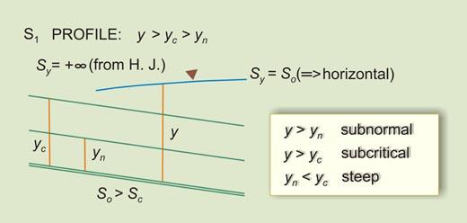
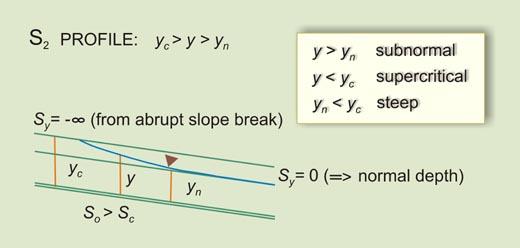
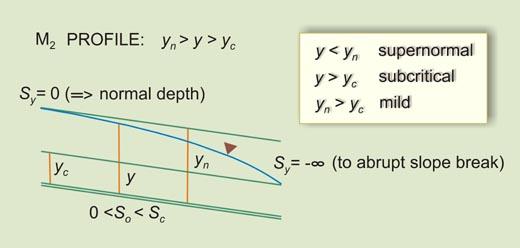
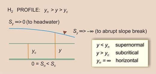
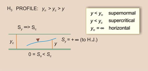
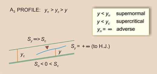
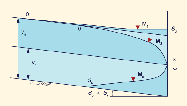
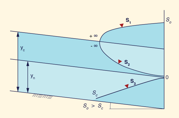
7.2 CHARACTERISTICS OF FLOW PROFILES
In Eq. 7-25, the sign of the left-hand side (LHS) is that of Sy
(numerator), since Sc (denominator)
is always positive (friction is always positive). The sign of Sy (i.e, the sign of
the LHS) may be one of three possibilities:
- A positive value, leading to RETARDED FLOW (BACKWATER),
- A zero value, leading to UNIFORM FLOW (NORMAL), or
- A negative value, leading to ACCELERATED FLOW (DRAWDOWN).
In the right-hand side (RHS) of Eq. 7-25, there are three possibilities for the numerator (USDA Soil Conservation Service, 1971):
- So / Sc > F 2, leading to SUBNORMAL FLOW,
- So / Sc = F 2, leading to NORMAL FLOW, or
- So / Sc < F 2, leading to SUPERNORMAL FLOW.
There are three possibilities for the denominator:
- 1 > F 2, leading to SUBCRITICAL FLOW,
- 1 = F 2, leading to CRITICAL FLOW, or
- 1 < F 2, leading to SUPERCRITICAL FLOW.
Given the above inequalities,
there arise three types (or families) of water-surface profiles, shown in Table 7-1.
The total number of profiles is 12.
A summary is shown in Table 7-2.
Table 7-1 Types of water-surface profiles.
| Type | Description
| Numerator and denominator of RHS
of Eq. 7-25 |
Sign
of
LHS | Flow
profile
|
I
| Subnormal/subcritical flow |
Both numerator and denominator are positive
|
+ |
Retarded | |
II | A
| Subnormal/supercritical flow | Numerator is positive and denominator is negative |
- |
Accelerated | | B | Supernormal/subcritical flow | Numerator is negative and denominator is positive |
- |
Accelerated | |
III | Supernormal/supercritical flow
| Both numerator and denominator are negative |
+ |
Retarded |
Table 7-2 Summary of water-surface profiles.
| Family
| Character
| Rule
| So > Sc
| So = Sc
| So < Sc
| So = 0
| So < 0
| I
| Retarded
(Backwater)
| 1 > F 2 < (So / Sc)
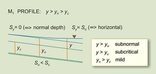
| S1
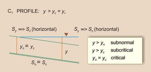
| C1
| M1
| -
| -
|
| II | A
| Accelerated
(Drawdown)
| 1 < F 2 < (So / Sc)
| S2
| -
| -
| -
| -
|
| B
| Accelerated
(Drawdown)
| 1 > F 2 > (So / Sc)
| -
| -
| M2
| H2
| A2
|
| III
| Retarded
(Backwater)
| 1 < F 2 > (So / Sc)
| S3
| C3
| M3
| H3
| A3
|
| |
|
Type I
In the Type I family, the flow is subnormal/subcritical. Therefore, the rule is:
1 > F 2 <
(So / Sc )
| (7-26) |
which is the same as:
Equation 7-27 states that So may be lesser than, equal to, or greater than Sc .
This gives rise to three types of profiles:
Since
and
it follows that
Thus:
Therefore, no horizontal (H) or adverse (A) profiles are possible in the Type I family of water-surface profiles.
|
|
Type II A
In the Type II A family, the flow is subnormal/supercritical. Therefore, the rule is:
1 < F 2 <
(So / Sc )
| (7-32) |
which is the same as:
Equation 7-33 states that So may only be greater than Sc . This gives rise
to only one profile:
Since
and
it follows that
Thus:
Therefore, no horizontal (H) or adverse (A) profiles are possible in the Type II A family of water-surface profiles.
|
|
Type II B
In the Type II B family, the flow is supernormal/subcritical. Therefore, the rule is:
1 > F 2 >
(So / Sc )
| (7-38) |
which is the same as:
Equation 7-39 states that So may be lesser than Sc ,
equal to 0, or lesser than 0.
This gives rise to three types of profiles:
|
|
Type III
In the Type III family, the flow is supernormal/supercritical. Therefore, the rule is:
1 < F 2 >
(So / Sc )
| (7-44) |
which is the same as:
Equation 7-45 states that So may be lesser than, equal to, or greater than Sc .
This gives rise to five types of profiles:
|
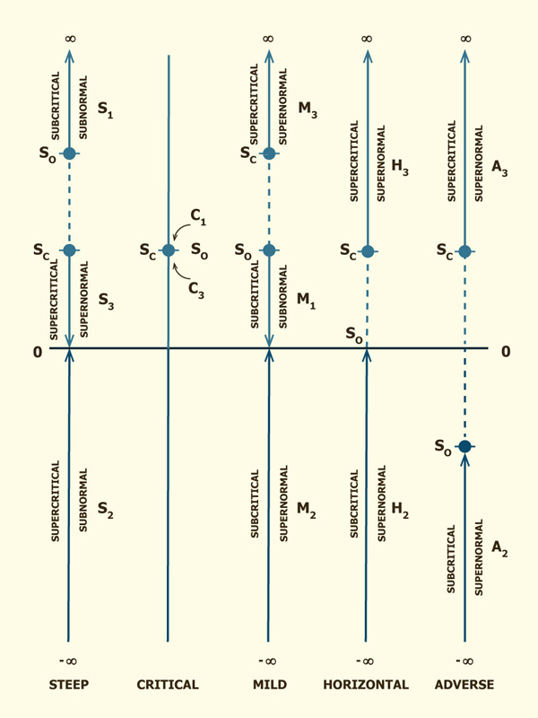
Figure 7-15 shows a graphical representation of flow-depth gradients
in water-surface profile computations. The
arrows indicate the direction of computation.
|
Fig. 7-15 Graphical representation of flow-depth gradient
ranges
in water-surface profile computations.
|
|
7.3 LIMITS TO WATER SURFACE PROFILES
The flow-depth gradients vary between five (5) limits (Fig. 7-15):
The channel slope So
The critical slope Sc
Zero.
+ ∞
- ∞
The theoretical limits to the water-surface profiles may be analyzed using Eq. 7-25, repeated
here in a slightly different form:
So - Sc F 2
Sy = ______________
1 - F 2
| (7-46) |
Operating in Eq. 7-46:
Sy (1 - F 2) = So - Sc F 2
| (7-47) |
So - Sy
F 2 = ____________
Sc - Sy
| (7-48) |
For uniform (normal) flow: Sy = 0, and Eq. 7-48 reduces to:
For gradually varied flow: Sy ≠ 0, and Eq. 7-48 is subject to three (3) cases:
-
F 2 > 0
So > Sy and Sc > Sy
The following inequality is satisfied: So > Sy < Sc
So < Sy and Sc < Sy
The following inequality is satisfied: So < Sy > Sc
It is concluded that Sy has to be either less than
both So and Sc, or greater than both.
|
F 2 < 0: Since F ≥ 0, this condition is impossible.
The following inequality is NOT satisfied: So > Sy > Sc
The following inequality is NOT satisfied: So < Sy < Sc
It is concluded that Sy cannot be less than So and greater than
Sc , or
less than Sc and greater than
So
. Thus, Sy has to be less than both So AND Sc,
or greater than both (See Case 1).
|
Uses of water-surface profiles
Table 7-3 and Fig. 7-17 show the typical occurrence of mild water-surface profiles.
|
Table 7-3 Occurrence of mild water-surface profiles. |
| M1
| Flow in a mild channel, upstream of a reservoir.
|
| M2
| Flow in a mild channel, upstream of an abrupt change in grade or a steep channel carrying supercritical flow.
|
| M3
|
Flow in a mild channel, downstream of a steep channel carrying supercritical flow.
|
|
Fig. 7-17 Typical occurrence of mild profiles.
|
|
Table 7-4 and Fig. 7-18 show the typical occurrence of steep water-surface profiles.
|
Table 7-4 Occurrence of steep water-surface profiles. |
| S1
| Flow in a steep channel, upstream of a reservoir.
|
| S2
|
Flow in a steep channel, downstream of a mild channel carrying subcritical flow.
|
| S3
| Flow in a steep channel,
downstream of a steeper channel carrying supercritical flow.
|
|
Fig. 7-18 Typical occurrence of steep profiles.
|
|
7.4 METHODOLOGIES
There are two ways to calculate water-surface profiles:
The direct step method.
The standard step method.
The direct step method is applicable to prismatic channels, while the standard step method
is applicable to any channel, prismatic and nonprismatic (Table 7-5). The direct step method is direct,
readily amenable to use with a spreadsheet, and relatively straight forward in its solution.
The standard step method is iterative and complex
in its solution. In practice, the standard step method is represented by the Hydrologic Engineering Center's
River Analysis System, referred to as HEC-RAS
(U.S. Army Corps of Engineers, 2020).
The direct step method applies particularly where
data is scarce and resources are limited.
The standard step method applies for comprehensive projects. The use of a widely accepted government program
such as HEC-RAS enhances credibility.
The required number of cross sections in the standard step method increases with the channel slope.
Steeper channels may require more cross sections. Lesser cross sectional variability
results in more reliable and accurate results. Note that extensive two- and three-dimensional flow features
may not be accurately represented in the one-dimensional water-surface profile model.
|
Table 7-5 Comparison between direct step and standard step methods. |
| No. | Characteristic | Direct step method |
Standard step method |
| 1 | Cross-sectional shape | Prismatic |
Any (prismatic or nonprismatic) |
| 2 | Ease of computation | Easy (hours) |
Difficult (months) |
| 3 | Calculation advances ⇒ | Directly |
By iteration (trial and error) |
| 4 | Type of cross-section input | One typical
cross section (prismatic) |
Several cross sections (nonprismatic) |
| 5 | Data needs | Minimal |
Extensive | | 6 | Accuracy increases with ↠ | A smaller flow depth increment |
More cross sections and/or lesser cross-sectional variability |
| 7 | Independent variable | Flow depth |
Length of channel |
| 8 | Dependent variable | Length of channel |
Flow depth |
| 9 | Tools | Spreadsheet or programming |
HEC-RAS |
| 10 | Reliability | Answer is always possible |
Answer is sometimes not possible, depending
on the type of cross-sectional input data |
| 11 | Cost | Comparatively small |
Comparatively large |
| 12 |
Public acceptance | Average |
High |
7.5 DIRECT STEP METHOD EXAMPLE
Calculation of M2 and S2 profiles, upstream and downstream
of a change in grade, from mild to steep
Input data:
- Discharge Q = 2000 m3/s
- Bottom width b = 100 m.
- Side slope 2 H : 1 V
- Upstream channel slope = 0.0001
- Upstream channel Manning's n = 0.025
- Downstream channel slope = 0.03
- Downstream channel Manning's n = 0.045
Solution
Calculate the normal depth and velocity,
and critical depth and velocity, in the upstream and downstream channels.
Use ONLINE CHANNEL 05.
For the upstream channel:
Normal depth = 10.098 m
Normal velocity = 1.648 m/s
Normal Froude number = 0.179
Critical depth = 3.364 m
Critical velocity = 5.571 m/s
For the downstream channel:
Normal depth = 2.669 m
Normal velocity = 7.113 m/s
Normal Froude number = 1.425
Critical depth = 3.364 m
Critical velocity = 5.571 m/s
Calculation of critical slope for the upstream channel:
yc = 3.364 m
Vc = 5.571 m/s
Ac = (b + zyc ) yc = 359.033 m2
Pc = b + 2 yc (1 + z 2)1/2 = 115.044 m
Rc = Ac / Pc = 3.121 m
Sc = n 2 Vc2 / Rc4/3 = (0.025)2
(5.571)2 (3.121)4/3 = 0.00425
Verify the critical slope with ONLINE CHANNEL 04: Sc = 0.004254.
Calculation of critical slope for the downstream channel:
Sc = n 2 Vc2 / Rc4/3 = (0.045)2
(5.571)2 (3.121)4/3 = 0.0138
Verify the critical slope with ONLINE CHANNEL 04: Sc = 0.01378.
The calculation of the M2 water-surface profile is shown in Table 7-6.
The following instructions are indicated:
The calculation moves in the upstream direction, starting at critical depth at the downstream end.
Column [1]: The second depth is set at 4 m; subsequently, the depth interval is set at 1 m.
Column [2]: The flow area is: A = (b + zy ) y . . . (1)
Column [3]: The mean velocity is: V = Q / A . . . (2)
Column [4]: The velocity head is: V 2 / (2g) . . . (3)
Column [5]: The specific head is: H = y + V 2 / (2g) . . . (4)
Column [6]: The wetted perimeter is: P = b + 2 y (1 + z 2)1/2 . . . (5)
Column [7]: The hydraulic radius is: R = A / P . . . (6)
Column [8]: The friction slope is: Sf = n 2 V 2 / R 4/3 . . . (7)
Column [9]: The average friction slope is: Sf ave = 0.5 (Sf 1
+ Sf 2) . . . (8)
Column [10]: The specific head difference is: ΔH = H2 - H1 . . . (9)
Column [11]: The channel length increment ΔL,
explained in the box below.
Column [12]: The cumulative channel length, i.e., the cumulative sum of ΔL increments.
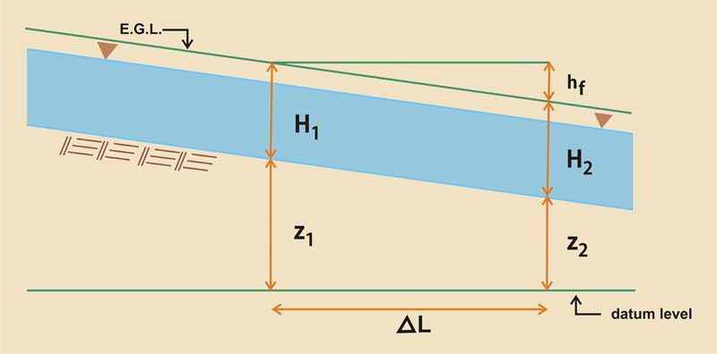
Derivation of the formula for the channel length increment ΔL
With reference to Fig. 7-19, the average friction slope is:
hf
Sf ave = ______
ΔL
| (7-54) |
|
Fig. 7-19 Definition sketch for the calculation of channel length increment ΔL.
|
|
H1 +
z1 = H2 +
z2 + Sf ave ΔL
| (7-55) |
z1 -
z2 = H2 -
H1 + Sf ave ΔL
| (7-56) |
z1 -
z2 - Sf ave ΔL = H2 -
H1
| (7-57) |
z1 -
z2
So = _________
ΔL
| (7-58) |
So ΔL - Sf ave ΔL = H2 -
H1
| (7-59) |
(So - Sf ave) ΔL = H2 -
H1
| (7-60) |
H2 -
H1
ΔL = ______________
So - Sf ave
| (7-61) |
ΔH
ΔL = ______________
So - Sf ave
| (7-62) |
Equation 7-62 enables the calculation of the channel length increment ΔL, i.e., Col. 11 of Table 7-6.
When ΔL is negative, the calculation moves upstream, as in the M2 profile (Table 7-6).
Conversely, when ΔL is positive, the
calculation moves downstream, as in the S2 profile (Table 7-7).
|
|
Table 7-6 Calculation of M2 water-surface profile (So = 0.0001). |
| [1]
| [2]
| [3]
| [4]
| [5]
| [6]
| [7]
| [8]
| [9]
| [10]
| [11]
| [12]
|
| y
| A
| V
| V 2/(2g )
| H
| P
| R
| Sf
| Sf ave
| ΔH
| ΔL
| ∑ ΔL
|
|
| (1)
| (2)
| (3)
| (4)
| (5)
| (6)
| (7)
| (8)
| (9)
| Box
|
|
| 3.364
| 359.033
| 5.570
| 1.581
| 4.945
| 115.044
| 3.1208
| 0.00425
| ---
| ---
| ---
| 0
|
| 4.000
| 432.000
| 4.630
| 1.092
| 5.092
| 117.888
| 3.664
| 0.00237
| 0.00331
| 0.147
| -45.794
| -45.794
|
| 5.000
| 550.000
| 3.636
| 0.674
| 5.674
| 122.360
| 4.495
| 0.00111
| 0.00174
| 0.528
| -354.878
| -400.672
|
| 6.000
| 672.000
| 2.976
| 0.451
| 6.451
| 126.833
| 5.298
| 0.00060
| 0.000855
| 0.777
| -1029.139
| -1429.811
|
| 7.000
|
|
|
|
|
|
|
|
|
|
|
|
| 8.000
|
|
|
|
|
|
|
|
|
|
|
|
| 9.000
|
|
|
|
|
|
|
|
|
|
|
|
| 10.000
|
|
|
|
|
|
|
|
|
|
|
|
| 10.097
|
|
|
|
|
|
| 0.0001
|
|
|
|
|
In the direct step method, the accuracy of the computation depends on the size of depth interval (Col. [1] of Table 7-6).
The smaller the interval, the more accurate the computation will be. This is because the average friction slope for a subreach (Col. [9])
is the arithmetic average of the friction slopes at the grid points (linear assumption). In practice, a computation
using a computer would have a much finer interval than that shown in Table 7-6.
The calculation of the S2 water-surface profile is shown in Table 7-7.
|
Table 7-7 Calculation of S2 water-surface profile (So = 0.03). |
| [1]
| [2]
| [3]
| [4]
| [5]
| [6]
| [7]
| [8]
| [9]
| [10]
| [11]
| [12]
|
| y
| A
| V
| V 2/(2g )
| H
| P
| R
| Sf
| Sf ave
| ΔH
| ΔL
| ∑ ΔL
|
|
| (1)
| (2)
| (3)
| (4)
| (5)
| (6)
| (7)
| (8)
| (9)
| Box
|
|
| 3.364
| 359.033
| 5.570
| 1.581
| 4.945
| 115.044
| 3.1208
| 0.00425
| ---
| ---
| ---
| 0
|
| 3.300
| 351.780
| 5.685
| 1.647
| 4.9475
| 114.758
| 3.0654
| 0.0147
| 0.01425
| 0.002
| 0.127
| 0.127
|
| 3.200
| 340.48
| 5.874
| 1.759
| 4.9586
| 114.311
| 2.979
| 0.0163
| 0.0155
| 0.0111
| 0.765
| 0.892
|
| 3.100
| 329.22
| 6.075
| 1.881
| 4.981
| 113.864
| 2.891
| 0.0181
| 0.0172
| 0.0224
| 1.750
| 2.642
|
| 3.000
|
|
|
|
|
|
|
|
|
|
|
|
| 2.900
|
|
|
|
|
|
|
|
|
|
|
|
| 2.800
|
|
|
|
|
|
|
|
|
|
|
|
| 2.700
|
|
|
|
|
|
|
|
|
|
|
|
| 2.669
|
|
|
|
|
|
| 0.03
|
|
|
|
|
Online calculations
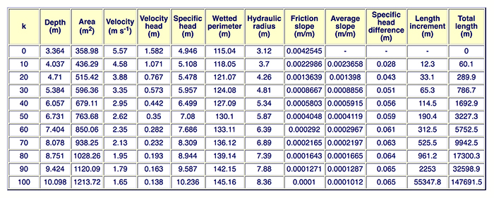
The M2 water-surface profiles (Fig. 7-20) may be calculated online using ONLINE_WSPROFILES_22.
Using the number of computational intervals n = 100, and number of tabular output intervals m = 100,
the length of the M2 water-surface profile is calculated to be: ∑ ΔL = 147,691.5 m. (Fig. 7-21).
|
Fig. 7-20 Definition sketch for M2 water-surface profile.
|
|
|
Fig. 7-21 Tabular result of ONLINE_WSPROFILES_22.
|
|
The S2 water-surface profiles (Fig. 7-22) may be calculated online using ONLINE_WSPROFILES_25.
Using the number of computational intervals n = 100, and number of tabular output intervals m = 100,
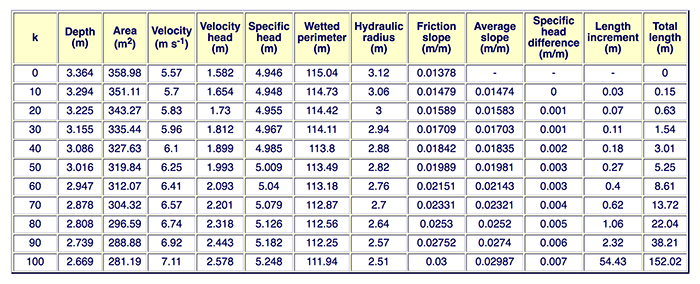
the length of the S2 water-surface profile is calculated to be: ∑ ΔL = 152.02 m (Fig. 7-23).
|
Fig. 7-22 Definition sketch for S2 water-surface profile.
|
|
|
Fig. 7-23 Tabular result of ONLINE_WSPROFILES_25.
|
|
7.6 CHANNEL TRANSITIONS
A transition is an open-channel flow structure whose purpose is to change the shape or cross-sectional area of the flow.
The design objective is to avoid excessive energy losses and to minimize surface waves and other turbulence.
When the transition is designed to keep the streamlines smooth and parallel, the theory of gradually varied flow is applicable.
In practice, the design of channel transitions is based
on the principles of energy and momentum conservation.
The form or shape of a transition may vary from as simple as straight-line headwalls normal to the flow to very elaborate
streamlined warped structures. Straight-line headwalls are often satisfactory for small canal structures or
where there is plenty of available hydraulic head (Fig. 7-24).
Other simplifications may be applied as long as they do not cause excessive wave action or turbulence (Fig. 7-25).
Fig. 7-24 A simple channel transition.
Common types of transitions are inlet and outlet transitions between: (1) canal and flume, (2) canal and tunnel, and (3)
canal and inverted siphon. Appreciable changes in flow depth within the transition may lead to rapidly varied flow
and the generation of standing waves.
| [Click on figure to display] |
Fig. 7-25 Typical flume inlets and outlets (Hinds, 1928).
Careful consideration should be given to the detail dimensions of the transition
throughout its entire length. The design water-surface profile
should be a smooth, continuous curve,
tangent to the water-surface profile upstream and downstream of the transition.
In general, it is desirable to avoid either critical flow or a hydraulic jump within the transition. An example of a channel transition from supercritical to subcritical flow,
with and without a hydraulic jump is given in
Section 3.6.
A curved transition should be used in all
important designs.
The best approach is to first select the shape of the water surface
and then to calculate the dimensions of the
cross sections to conform with established principles of conservation of energy.
Transition between canal and flume, or canal and tunnel
The following design features are considered (Hinds, 1928; Chow, 1959):
Length and angle. A well-designed transition should avoid sharp angles to minimize the possibility of standing waves.
The optimum angle subtended between the channel axis and a line connecting the
channel sides between entrance and exit sections is 12.5°.
Losses. The energy loss through a transition has two components:
Conversion loss, which is generally expressed in terms of the change
in velocity head between the entrance and exit sections of the
transition structure. Table 7-8 shows conversion loss coefficients for transitions.
Friction loss, which may be estimated by the use of a uniform flow formula.
This loss is usually very small and may be considered negligible in a preliminary design.
Table 7-8 Conversion loss coefficients for transitions.
|
| Type of transition |
Inlet coefficient ci |
Outlet coefficient co |
| Warped |
0.10 |
0.20 |
| Cylinder quadrant |
0.15 |
0.25 |
| Simplified straight line |
0.20 |
0.30 |
| Straight line |
0.30 |
0.50 |
| Square ended |
0.30 + |
0.75 |
|
Water-surface profile.
The drop in water-surface elevation from end of the
canal to
midlength of the transition should be equal to half of the total drop through the entire length.
From canal end to midlength, the individual drops should be proportional to the square of the distance (a forward parabola).
From midlength to beginning of flume, the drops should mirror those of the first half-length, in reverse order (a backward parabola).
Using this procedure, a smooth curve is obtained for the water-surface profile.
Freeboard. The customary rules for the estimation of freeboard for lined and unlined canals may be used.
For flow depths exceeeding 12 ft (4 m), the freeboard should be examined carefully.
Energy loss in transitions
For inlet structures, the velocity at the entrance section is less than the velocity at the exit; hence, the water surface must drop
at least the full difference between the velocity heads plus a small conversion loss known as the inlet loss.
Therefore, the drop Δy' in water-surface elevation for an inlet structure is:
Δy' = Δhv + ci Δhv = ( 1 + ci ) Δhv
| (7-63) |
where Δhv is the velocity head difference between entrance and exit sections.
For outlet structures, the velocity at the entrance section is greater than the velocity at the exit; hence, the water surface must rise
to recover velocity head. The drop is equal to the full difference between the velocity heads minus a small conversion rise known as the outlet rise.
Therefore, the drop Δy' in water-surface elevation for an outlet structure is:
Δy' = Δhv - co Δhv = ( 1 - co ) Δhv
| (7-64) |
Figure 7-26 shows the following typical designs: (a) an inlet transition from canal to flume, and (b) an outlet transition from
flume to canal. The step-by-step design of an inlet transition between canal and flume is explained below.
The design of an outlet transition
follows the same general steps as in the case of the inlet transition. However, the outlet transition is often complicated due to the presence of uneven velocity distribution.
In this case, the velocity distribution coefficients may be appreciably greater than one (1) and, therefore, should be examined carefully.
| [Click on figure to display] |
Fig. 7-26 (a) Design of an inlet transition (Modified from Chow, 1959).
| [Click on figure to display] |
Fig. 7-26 (b) Design of an outlet transition (Chow, 1959).
Design of an inlet transition: Example
The following example was originally presented by Hinds (1928)
and subsequently cited by Chow (1959).
It is reproduced here with detailed explanation and minor corrections for rounding accuracy. |
Design an inlet transition to connect
an unlined canal of bottom width b = 18 ft and side slope
z = 2 H: 1 V, with a rectangular concrete flume
of width b = 12.5 ft. The hydraulic conditions are:
Design discharge: Q = 314.5 cfs
Canal bottom slope: S = 0.000246
Manning's n of canal: n = 0.018
Flume bottom slope: S = 0.0009
Manning's n of flume: n = 0.014
Water-surface elevation
immediately upstream of the transition, at Station 0 + 00: Zw,0 = 57.410 ft.
Table 7-9 shows the hydraulic
properties of the canal and flume, corresponding to normal flow: depth yn (ft),
velocity Vn (fps),
flow area An (sq. ft.),
wetted perimeter Pn (ft),
top width Tn (ft),
hydraulic radius Rn (ft), and
hydraulic depth Dn (ft). The hydraulic properties were calculated
using
onlinechannel01.
Table 7-9 Hydraulic properties of the canal and flume.
|
| Type |
b |
z |
S |
n |
yn |
Vn |
An |
Pn |
Tn |
Rn |
Dn |
| Canal |
18.0 |
2 |
0.000246 |
0.018 |
4.311 |
2.74 |
114.77 |
37.28 |
35.244 |
3.079 |
3.256 |
| Flume |
12.5 |
0 |
0.0009 |
0.014 |
4.254 |
5.914 |
53.18 |
21.008 |
12.5 |
2.531 |
4.254 |
|
Solution Procedure
-
Length of the transition.
To determine the length of the transition, a straight line
joining the flow line (on the wall) at the two ends of the transition
should make an angle θ = 12.5° with the longitudinal alignment.
The length of the transition is equal to half of the difference between the normal top widths of canal and flume,
divided by tan θ:
L =
0.5 ( Tn canal - Tn flume ) / tan θ
| (7-65a) |
L =
0.5 (35.244 - 12.5) / 0.2217 = 51.3 ft
| (7-65b) |
Assume L = 50 ft as a round number to be used for design.
Difference in velocity head.
The velocity head at the upstream cross section (end of canal) is:
hv = (2.74)2 / (2 × 32.17) = 0.117 ft
| (7-66b) |
Likewise, the velocity head at the downstream cross section (beginning of flume) is: hv = 0.544 ft.
The velocity head difference is:
Δhv =
0.544 - 0.117 = 0.427 ft.
| (7-67) |
Energy losses, neglecting
friction. For a warped transition,
shown in Fig. 7-26 (a),
the inlet loss coefficient is ci = 0.1 (Table 7-8).
Therefore, the total drop in water-surface elevation, neglecting frictional losses, is (Eq. 7-63):
Δy' =
1.1 × 0.427 = 0.470 ft.
| (7-68) |
Calculation of drop in water-surface elevation.
The water-surface
elevation (water-surface profile) may be approximated as two equal parabolas, pieced together at midpoint of the transition,
positioned in such a way that the forward parabola is
tangent to the flow at the end of the canal, and the backward parabola is tangent to the flow at the
start of the flume. The two parabolas are tangent to themselves at midpoint of the
transition (Hinds, 1928). The following drops are fixed:
- At the upstream section, Station 0 + 00,
the drop is: Δy'0 = 0.000 ft;
- At midlength, Station 0 + 25, the drop is half the
full drop, i.e., Δy'5 = 0.235 ft; and
- At the downstream section, Station 0 + 50,
the drop is the full drop: Δy'10 = 0.470 ft.
Assume that the length L of the transition is divided into n = 10
equal subreaches, making a total of eleven (11) stations or cross sections, at a distance of 5-ft apart.
To calculate the drops, define a as the half-length of the transition;
thus, a = 25 ft. Furthermore, define b as one-half of the total drop in water-surface elevation Δy'.
Thus, b = 0.235 ft.
For each station i, the forward parabola is defined by varying i from 1 to 4 as follows:
Δy'i =
(b /a 2) xi 2
| (7-69a) |
For instance, for i = 1:
Δy'1 =
(0.235 / 25 2) 5 2 = 0.0094 ≅ 0.009
| (7-69b) |
The backward parabola is defined by varing i from 9 to 6 as follows:
Δy'i =
Δy'10 -
Δy'10 - i
| (7-69c) |
For instance, for i = 9:
Δy'9 =
Δy'10 -
Δy'1 = 0.470 - 0.009 = 0.461
| (7-69d) |
Similarly, for i = 8:
Δy'8 =
Δy'10 -
Δy'2 = 0.470 - 0.038 = 0.432
| (7-69e) |
Table 7-10 shows the partial drop in
water-surface elevation Δy'i corresponding to
each station i, calculated using Eq. 7-69.
These values are inserted in Col. 2 of Table 7-11.
Table 7-10 Calculation of drop in water-surface elevation.
|
| Station |
0+00 |
0+05 |
0+10 |
0+15 |
0+20 |
0+25 |
0+30 |
0+35 |
0+40 |
0+45 |
0+50 |
| i |
0 |
1 |
2 |
3 |
4 |
5 |
6 |
7 |
8 |
9 |
10 |
| xi (ft) |
0 |
5 |
10 |
15 |
20 |
25 |
30 |
35 |
40 |
45 |
50 |
| Δy'i (ft) |
0.000 |
0.009 |
0.038 |
0.085 |
0.150 |
0.235 |
0.320 |
0.385 |
0.432 |
0.461 |
0.470 |
|
The computational procedure consists of the following steps, detailed in Table 7-11 below:
Column 1 shows the eleven (11) stations, from Station 0 + 00 to Station 0 + 50.
Column 2 shows the partial drops in water-surface elevation Δy'.
Column 3 shows the change in velocity head Δhv,
equal to the value of Col. 2 divided by 1.1 (from Eq. 7-68).
Column 4 shows the velocity heads at each cross section,
beginning with 0.117 ft at the upstream end (Sta. 0 + 00) to 0.544 ft at the downstream end (Sta. 0 + 50).
To calculate the values of Col. 4, for each station, the values of Col. 3 are added to the value for Col. 4, Sta. 0 + 00 (0.117).
Column 5 shows the velocity V corresponding to the velocity head hv of Col. 4:
V = (2 × 32.17 × hv)1/2
| (7-70b) |
Column 6 shows the flow area A, obtained by dividing the discharge (Q = 314.5 cfs) by the corresponding velocity of Col. 5.
Column 7 shows half the top width 0.5 T,
obtained from the sketched plan [(Fig. 7-24 (a)].
The plan may be chosen arbitrarily or by trial,
until satisfactory results are obtained (Chow, 1959).
The values shown here are those of the original example (Hinds, 1928).
Column 8 shows half the bottom width 0.5 b, obtained from the cross sections of the sketched plan [(Fig. 7-24 (a)]. The values shown here are those of the original example (Hinds, 1928).
Column 9 shows the flow depth y, calculated as follows:
y = A / (0.5 T + 0.5 b).
| (7-71) |
Note that at the downstream end of the
transition, the flow depth for Sta. 0 + 50 has been adjusted
to 4.254 ft.
Column 10 shows the wetted perimeter P, calculated as follows:
P = 2 { 0.5 b + [ ( 0.5 T - 0.5 b )2 + y 2 ] 0.5 }
| (7-72) |
Column 11 shows the hydraulic radius:
Column 12 shows the friction slope,
calculated using the Manning equation:
V = ( 1.486 / n ) R 2/3 Sf 1/2
| (7-74) |
Therefore:
Sf = 0.45286 V 2 n 2 R - 4/3
| (7-75) |
in which n = 0.014 (the flume value) is used for all sections in the transition.
Column 13 shows the incremental friction head loss Δhf between two
adjoining sections, calculated as the equidistance (5 ft) multiplied by the average friction slope for the indicated reach:
Column 14 shows the cumulative friction head loss ∑ Δhf.
| Table 7-11 (a) Tabular computation for the design of an inlet transition. |
| (1) |
(2) |
(3) |
(4) |
(5) |
(6) |
(7) |
(8) |
(9) |
(10) |
(11) |
(12) |
(13) |
(14) |
| Variable |
Δy' |
Δhv |
hv |
V |
A |
0.5 T |
0.5 b |
y |
P |
R |
Sf |
Δhf |
∑ Δhf |
| Station |
(ft) |
(ft) |
(ft) |
(fps) |
(ft2) |
(ft) |
(ft) |
(ft) |
(ft) |
(ft) |
|
(ft) |
(ft) |
| 0 + 00 |
0.000 |
0.000 |
0.117 |
2.740 |
114.771 |
17.600 |
9.000 |
4.315 |
37.243 |
3.082 |
0.000150 |
- |
- |
| 0 + 05 |
0.009 |
0.009 |
0.125 |
2.839 |
110.790 |
17.000 |
8.625 |
4.324 |
36.100 |
3.069 |
0.000160 |
0.000773 |
0.000773 |
| 0 + 10 |
0.038 |
0.034 |
0.151 |
3.116 |
100.947 |
15.427 |
7.917 |
4.324 |
33.166 |
3.044 |
0.000200 |
0.000889 |
0.001662 |
| 0 + 15 |
0.085 |
0.0777 |
0.194 |
3.529 |
89.120 |
13.460 |
7.250 |
4.303 |
29.611 |
3.010 |
0.000250 |
0.001124 |
0.002786 |
| 0 + 20 |
0.150 |
0.137 |
0.253 |
4.037 |
77.900 |
11.228 |
6.958 |
4.284 |
26.013 |
2.995 |
0.000340 |
0.001474 |
0.004260 |
| 0 + 25 |
0.235 |
0.213 |
0.330 |
4.609 |
68.235 |
9.139 |
6.771 |
4.289 |
23.340 |
2.923 |
0.000450 |
0.001966 |
0.006226 |
| 0 + 30 |
0.319 |
0.290 |
0.407 |
5.117 |
61.457 |
7.717 |
6.667 |
4.273 |
22.133 |
2.777 |
0.000600 |
0.002617 |
0.008842 |
| 0 + 35 |
0.385 |
0.350 |
0.467 |
5.480 |
57.387 |
6.847 |
6.563 |
4.279 |
21.704 |
2.644 |
0.000730 |
0.003312 |
0.012154 |
| 0 + 40 |
0.432 |
0.393 |
0.509 |
5.725 |
54.930 |
6.458 |
6.458 |
4.253 |
21.422 |
2.564 |
0.000830 |
0.003895 |
0.016050 |
| 0 + 45 |
0.460 |
0.418 |
0.535 |
5.868 |
53.599 |
6.315 |
6.315 |
4.244 |
21.118 |
2.538 |
0.000880 |
0.004279 |
0.020329 |
| 0 + 50 |
0.470 |
0.427 |
0.544 |
5.914 |
53.177 |
6.250 |
6.250 |
4.254 |
21.008 |
2.531 |
0.000900 |
0.004457 |
0.024786 |
|
Column 15 [Table 7-11 (b)] shows the water-surface elevation.
At Station 0 + 00: Zw,0 = 57.410 ft.
For each cross section i, the water-surface elevation is:
Zw,i = Zw,0 -
Δy'i - ∑ Δhf,i
| (7-77) |
Column 16 shows the channel bottom elevation.
For each cross section i, the channel bottom elevation is:
Column 17 shows the side slope z, calculated as follows:
z = (0.5 T - 0.5 b) / y
| (7-79) |
Column 18 shows the elevation of the top of lining ZL.
To facilitate construction of the lining, the elevation ZL makes a straight line through the transition.
The recommended height of lining above the water surface for Q = 314.5 cfs is about 1 ft.
Accordingly, the value of ZL at midpoint of the transition (Sta. 0 + 25) should be:
ZL (Sta. 0 + 25) = Zw (Sta. 0 + 25) + 1
| (7-80a) |
ZL (Sta. 0 + 25) = 57.169 + 1 = 58.169
| (7-80b) |
The total drop in water-surface elevation
through the transition is [Table 7-11 (b), Col. 15]:
ΔZw = 57.410 - 56.915 = 0.495
| (7-81) |
Within any two adjacent cross sections, the drop in water-surface elevation is: 0.495/10 = 0.0495.
Therefore, the elevation of the top of lining upstream of the transition is:
ZL (Sta. 0 + 00) = 58.169 + (5 × 0.0495) = 58.416
| (7-82) |
Likewise, the elevation of the top of lining downstream of the transition is:
ZL (Sta. 0 + 50) = 58.169 - (5 × 0.0495) = 57.922
| (7-83) |
The values of ZL for the remaining cross sections are obtained by linear interpolation.
Column 19 shows the height of the lining HL, calculated as follows:
Column 20 shows the computed values of
the half-width 0.5 W, measured at the top of the lining:
0.5 W = z HL + 0.5 b
| (7-85) |
Column 21 shows the adopted
value of the half-width 0.5 W, measured at the top of the lining.
The values of Col. 21 are indicated in the plan view shown in
Fig. 7-26 (a).
| Table 7-11 (b) Tabular computation for the design of an inlet transition (continued). |
| (1) |
(15) |
(16) |
(17) |
(18) |
(19) |
(20) |
(21) |
| Variable |
Zw |
Zb |
z |
ZL |
HL |
0.5 W
(computed) |
0.5 W
(adopted) |
| Station |
(ft) |
(ft) |
z H: 1 V |
(ft) |
(ft) |
(ft) |
(ft-in) |
| 0 + 00 |
57.410 |
53.095 |
1.993 ≅ 2 |
58.416 |
5.321 |
19.605 |
19'-8" |
| 0 + 05 |
57.400 |
53.076 |
1.937 |
58.367 |
5.290 |
18.873 |
18'-11" |
| 0 + 10 |
57.371 |
53.046 |
1.737 |
58.317 |
5.271 |
17.071 |
17'-1.5" |
| 0 + 15 |
57.323 |
53.019 |
1.443 |
58.268 |
5.248 |
14.824 |
14'-10" |
| 0 + 20 |
57.255 |
52.972 |
0.997 |
58.218 |
5.246 |
12.188 |
12'-2" |
| 0 + 25 |
57.169 |
52.880 |
0.552 |
58.169 |
5.289 |
9.691 |
9'-8.5" |
| 0 + 30 |
57.082 |
52.809 |
0.246 |
58.120 |
5.310 |
7.972 |
7'-11.5" |
| 0 + 35 |
57.013 |
52.733 |
0.066 |
58.070 |
5.337 |
6.917 |
6'-11" |
| 0 + 40 |
56.962 |
52.709 |
0 |
58.021 |
5.312 |
6.458 |
6'-5.5" |
| 0 + 45 |
56.929 |
52.686 |
0 |
57.971 |
5.286 |
6.315 |
6'-4" |
| 0 + 50 |
56.916 |
52.661 |
0 |
57.922 |
5.260 |
6.250 |
6'-3" |
|
The design of a channel transition may be performed with the aid of the
onlinetransitiondesign.php
calculator featured in onlinecalc.sdsu.edu.
QUESTIONS
What is steady gradually varied flow?
What is retarded flow?
What is accelerated flow?
What is subnormal flow?
What is supernormal flow?
How many profiles are possible in steady gradually varied flow?
What is the rule for the Type I family of water-surface profiles?
What is the rule for the Type III family of water-surface profiles?
Which water-surface profiles are completely horizontal?
What are the five limits to the water surface profiles?
What is the typical application of the M1 water-surface profile?
What is the typical application of the S1 water-surface profile?
What is the typical application of the S3 water-surface profile?
What is the main difference between the direct-step and standard-step methods
of water-surface profile computations?
PROBLEMS
A perennial stream has the following properties: discharge
Q = 30 m3/s, bottom width b = 55 m, side slope z = 2,
bottom slope So = 0.0004, and Manning's n = 0.035.
A 2-m high diversion dam is planned on the stream to raise the head for an irrigation canal (Fig. 7-25).
- Calculate the normal depth.
- Calculate the total length of the M1 water-surface profile. Use n = 400 and m = 400.
- Calculate the partial length of the M1 profile,
from the dam to a location upstream where the normal depth is exceeded by 1%.
Use ONLINE CHANNEL 01
and ONLINE WSPROFILES 21.
|
Fig. 7-25 A diversion dam.
|
|
A perennial stream has the following properties: discharge
Q = 1000 ft3/s, bottom width b = 150 ft, side slope z = 2,
bottom slope So = 0.00038, and Manning's n = 0.035.
A 6-ft high diversion dam is planned on the stream to raise the head for an irrigation canal.
- Calculate the normal depth.
- Calculate the total length of the M1 water-surface profile. Use n = 400 and m = 400.
- Calculate the partial length of the M1 profile,
from the dam to a location upstream where the normal depth is exceeded by 1%.
Use ONLINE CHANNEL 01
and ONLINE WSPROFILES 21.
A mild stream flows into a steep channel, producing an M2
upstream of the brink. The hydraulic conditions in the channel are:
Q = 28 m3/s, bottom width b = 12 m, side slope z = 2.5,
bottom slope So = 0.0007, and Manning's n = 0.04.
Assume critical depth near the change in slope.
A mild stream flows into a steep channel, producing an M2
upstream of the brink. The hydraulic conditions in the channel are:
Q = 500 ft3/s, bottom width b = 30 ft, side slope z = 1.5,
bottom slope So = 0.00075, and Manning's n = 0.04.
Assume critical depth near the change in slope.
An overflow
spillway flows into a mild channel, producing a hydraulic jump.
The channel is rectangular, with Q = 3 m3/s, bottom width b = 8 m, and Manning's
n = 0.015.
The flow depth at the toe of the spillway is 0.1 m and the approximate slope at the toe of the spillway is 0.1.
The slope of the [mild] downstream channel, which functions as a stilling basin, is 0.0001.
Calculate:
- the critical depth,
- the length Ltc from the toe of the spillway to critical depth downstream,
- the Froude number at the toe of the spillway,
- the Froude number downstream of the hydraulic jump,
- the sequent depth y2 (the normal depth downstream of the hydraulic jump),
- the length Lj of the jump, assuming Lj = 6.2 y2
- the minimum length of the stilling basin Lsb = Ltc + Lj
Use ONLINE CHANNEL 02
and ONLINE WSPROFILES 23. In the latter, use n = 100 and m = 100.
An overflow
spillway flows into a mild channel, producing a hydraulic jump.
The channel is rectangular, with Q = 100 ft3/s, bottom width b = 20 ft, and Manning's
n = 0.015.
The flow depth at the toe of the spillway is 0.4 ft and the approximate slope at the toe of the spillway is 0.1.
The slope of the [mild] downstream channel, which functions as a stilling basin, is 0.0001.
Calculate:
- the critical depth,
- the length Ltc from the toe of the spillway to critical depth downstream,
- the Froude number at the toe of the spillway,
- the Froude number downstream of the hydraulic jump,
- the sequent depth y2 (the normal depth downstream of the hydraulic jump),
- the length Lj of the jump, assuming Lj = 6.2 y2
- the minimum length of the stilling basin Lsb = Ltc + Lj
Use ONLINE CHANNEL 02
and ONLINE WSPROFILES 23. In the latter, use n = 100 and m = 100.
A
diversion dam of height H = 1.8 m is planned on a steep stream with bottom slope
So = 0.035.
A hydraulic jump is expected upstream of the dam. Identify the type of water surface profile.
Using ONLINE CALC, calculate the length of the water surface profile,
from the location of the diversion dam, in the upstream direction, to
the [downstream end of the] hydraulic jump. The channel has
Q = 4 m3/s, bottom width b = 3 m, side slope z = 1,
and Manning's n = 0.03. What are the sequent depths?
What is the Froude number of the upstream flow? Use m = 100 and n = 100.
Verify the sequent depth y2
using ONLINE CHANNEL 11.
A mild channel enters into a steep channel
of slope So = 0.03.
Identify the type of water surface profile in the steep channel.
Using ONLINE CALC, calculate the normal depth in the steep channel,
and the length of the water surface profile to within 2% of normal depth.
The channel has
Q = 3 m3/s, bottom width b = 5 m, side slope z = 0,
and Manning's n = 0.015. What is the normal-depth Froude number in the steep channel?
Use m = 100 and n = 100.
A steep channel of slope So = 0.035 enters
into a milder steep channel of slope So = 0.012.
Identify the type of water surface profile in the milder steep channel.
Using ONLINE CALC, calculate the normal depth in the downstream channel,
and the length [to normal depth] of the water surface profile.
The channel has
Q = 3.2 m3/s, bottom width b = 4 m, side slope z = 2,
and Manning's n = 0.015. What are the normal-depth Froude numbers?
What is the normal depth in the upstream channel?
What would be the length of the water surface profile if Manning's n was instead estimated at 0.013? Use m = 100 and n = 100.
A perennial stream has the following properties: discharge
Q = 15 m3/s, bottom width b = 8 m, side slope z = 2,
bottom slope So = 0.0025, and Manning's n = 0.035.
A 2.0-m high diversion dam is planned on the stream to raise the head for an irrigation canal (Fig. 7-26).
- Calculate the normal depth.
- Calculate the total length of the M1 water-surface profile.
Use three resolutions: (a) n = 100 and m = 100, (b) n = 200 and m = 200,
and (c) n = 400 and m = 400.
Comment on the results.
- Using the higher resolution results, calculate the partial length of the M1 profile,
from the dam location to a point upstream where the normal depth is exceeded by 1%.
Use ONLINE CHANNEL 01
and ONLINE WSPROFILES 21.
|
Fig. 7-26 A diversion dam.
|
|
An overflow spillway flows into a mild channel, producing a hydraulic jump.
The channel is rectangular, with Q = 3.6 m3/s, bottom width b = 5 m, and Manning's n = 0.015.
The flow depth at the toe of the spillway is 0.15 m and the
approximate slope at the toe of the spillway is 0.1.
The slope of the downstream mild channel, which functions as a stilling basin, is 0.00016.
Use n = 100 and m = 100.
Calculate:
- the critical depth,
- the length Ltc from the toe of the spillway to critical depth downstream,
- the Froude number at the toe of the spillway,
- the Froude number downstream of the hydraulic jump,
- the sequent depth y2 (the normal depth downstream of the hydraulic jump),
- the length Lj of the jump, assuming Lj = 6.2 y2
- the minimum length of the stilling basin Lsb = Ltc + Lj
What would be the length of the stilling basin if the bottom width were to be increased to 7 m?
Use ONLINE CHANNEL 02
and ONLINE WSPROFILES 23. In the latter, use n = 100 and m = 100.
A 5-m high diversion dam is planned on a channel operating at critical flow.
The channel is rectangular, with
Q = 100 m3/s, bottom width b = 4.7 m,
bottom slope So = 0.01, and Manning's n = 0.023.
Calculate the length of the C1 water-surface profile.
Assume n = 100 and m = 100.
A steep channel, with bottom slope So = 0.03,
flows into a channel operating at critical flow.
The channel is rectangular, with
Q = 100 m3/s, bottom width b = 4.7 m, and Manning's n = 0.024.
Calculate the length of the C3 water-surface profile.
Assume n = 100 and m = 100.
A horizontal channel of length L = 500 m
is designed to convey Q = 5 m3/s
from a reservoir to a free overfall. The bottom width is b = 2 m, and side slope z = 1.5.
The channel is lined with gabions and the Manning's n recommended by the manufacturer is
n = 0.028.
- What is the headwater depth (accuracy to 1 cm)
required to pass the design discharge?
- What is the tailwater depth, that is, the critical flow depth at the downstream boundary?
Use ONLINE_WSPROFILES_28; assume n = 100 and m = 100.
A sluice gate is designed to release
supercritical flow into a stilling basin, where
a hydraulic jump will occur.
The basin channel bottom is horizontal, of rectangular cross section.
The design discharge is Q = 5 m3/s, the
bottom width b = 5 m, and Manning's n = 0.015.
Use
ONLINE_WSPROFILES_31; assume n = 100 and m = 100.
Assume So,u/s = 0.05 so that the flow through the sluice gate
remains supercritical.
A weir is located at the downstream end of a wide rectangular
channel of bottom slope So = 0.0035 and dimensionless Chezy friction factor
f = 0.0035.
The unit-width discharge in the wide rectangular channel is q = 0.4 m3/s/m. Immediately
upstream of the weir, the flow is subcritical, with depth y = 1.5 m.
What is the type and length of the water-surface profile immediately upstream of the weir?
A hydraulically wide channel with So = 0.025 flows
into a critical flow channel of So = 0.004. The dimensionless
Chezy friction factor f
is the same is both channels.
The unit-width discharge is 2.2 m3/s/m.
What is the type and length of the water-surface profile in the critical flow channel?
Design a warped inlet transition from canal to flume
for the following data: Design discharge = 300 cfs;
canal bottom width b = 12 ft;
canal side slope = 2 H : 1 V;
canal bottom slope = 0.0012;
canal Manning's n = 0.020;
flume bottom width b = 8 ft;
flume side slope = 0 H : 1 V;
flume bottom slope = 0.01;
flume Manning's n = 0.012;
water surface elevation immediately upstream of the transition Z = 100 ft.
Use the inverse parabolas option of ONLINE TRANSITION DESIGN.
REFERENCES
Chow, V. T. 1959. Open-channel Hydraulics. McGraw Hill, New York.
Hinds, J. 1928. Hydraulic design of flume and siphon transitions.
U.S. Bureau of Reclamation, 14 p.
U.S. Army Corps of Engineers. (2020). HEC-RAS: Hydrologic Engineering Center River Analysis System, Version 5.0.
USDA Soil Conservation Service. (1971). Classification system for varied flow in prismatic channels. Technical Release No. 47 (TR-47), Washington, D.C.
| http://openchannelhydraulics.sdsu.edu |
|
220530 |
| |
|