|
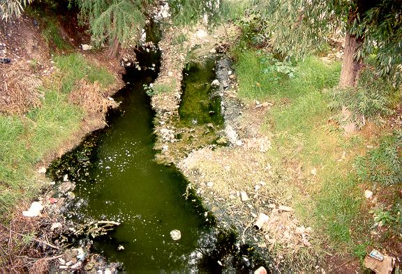
| Fig. 1 Sewage contamination of a small stream. |
Victor M. Ponce
Professor of Civil Engineering
San Diego State University
[110926]
ABSTRACT
The differential equation for the dissolved oxygen sag curve (DO sag curve) is derived. The solution of this differential equation can be shown to be essentially the same as that of the well known Streeter-Phelps equation (Streeter and Phelps, 1925). Unlike the latter, the differential equation derived herein can be solved numerically and, therefore, does not require integration. Moreover, the differential equation is valid for all deoxygenation and oxygenation constants, unlike the Streeter-Phelps equation, which is undefined when these constants are equal. Two online calculators: (a) single case, and (b) general case, round up the analysis.
1. INTRODUCTION
The discharge of a sewage effluent in a stream produces a biochemical oxygen demand (BOD) which decays exponentially in time and space.
This oxygen demand causes an oxygen deficit, or oxygen shortage. The greater the oxygen deficit,
the greater the rate of natural oxygen replenishment
from the atmosphere into the stream.
These two concurrent processes of oxygen consumption and oxygen replenishment
produce an oxygen sag curve, i.e., a curve which sags initially due to the
increased oxygen demand and recovers
asymptotically downstream due to the increased rate of oxygen replenishment. The derivation of the DO sag equation
is the objective of this article.
2. OXYGEN DEMAND
The exponential decay of oxygen demand can be modeled as follows (Tchobanoglous and Schroeder, 1985):
| D = Du e- kd t | (1) |
in which:
D = biochemical oxygen demand (BOD) (mg/liter);
Du = ultimate BOD immediately downstream of effluent discharge (mg/liter);
kd = deoxygenation constant (d-1);
t = time (d).
The differential equation for oxygen demand is:
| dD/dt = - kd Du e- kd t | (2) |
Using the chain rule, the oxygen demand equation is converted to the spatial domain:
| (dD/dx) (dx/dt ) = - kd Du e- kd t | (3) |
| dD/dx = - (kd /v ) Du e- (kd /v ) x | (4) |
in which:
x = distance along the stream, measured downstream of effluent discharge (m);
v = stream velocity (m/d).
3. ULTIMATE BOD
At the upstream boundary, a mass balance leads to:
| Du = ( Qs Ds + Qe De ) / (Qs + Qe ) | (5) |
in which:
Du = ultimate BOD immediately downstream of effluent discharge (mg/liter);
Qs = stream discharge (m3/s);
Ds = BOD in stream, immediately upstream of effluent discharge (mg/liter);
Qe = effluent discharge (m3/s);
De = BOD of effluent discharge (mg/liter);
Assuming the upstream flow is clean: Ds ≅ 0.
Therefore, the mass balance reduces to:
| Du = [ Qe / ( Qs + Qe ) ] De | (6) |
4. OXYGEN SUPPLY
The differential equation for oxygen supply in a stream can be modeled as follows (Tchobanoglous and Schroeder, 1985):
| dS/dt = ko (Ss - S ) | (7) |
in which:
ko = oxygenation constant (d-1);
Ss = dissolved oxygen concentration at saturation, a function of temperature, salinity, and atmospheric pressure (mg/liter); and
S = dissolved oxygen concentration (mg/liter).
The quantity (Ss - S ) is the oxygen deficit.
Using the chain rule, the oxygen supply equation is converted to the spatial domain:
| (dS/dx) (dx/dt) = ko (Ss - S ) | (8) |
Therefore:
| dS/dx = (ko /v ) (Ss - S ) | (9) |
5. DO SAG EQUATION
The change of dissolved oxygen concentration in space is given by the change in supply plus the change in demand:
| dO/dx = dS/dx + dD/dx | (10) |
in which O = dissolved oxygen concentration (mg/liter).
Combining Eqs. 4, 9, and 10:
| dO/dx = (ko /v ) (Ss - S ) - (kd /v ) Du e- (kd /v )x | (11) |
Since S = O:
| dO/dx = (ko /v ) (Ss - O ) - (kd /v ) Du e- (kd /v )x | (12) |
In a control volume (computational reach) of length L (m), with index j upstream
and
| (Oj+1 - Oj ) / L = (ko /v ) (Ss - Oj ) - (kd /v ) Du e- (kd /v )xj+1 | (13) |
Therefore:
| Oj+1 = Oj + L [ (ko /v ) (Ss - Oj ) - (kd /v ) Du e- (kd /v )xj+1 ] | (14) |
6. INITIAL DO
For j = 0: Oj = O0. At the upstream boundary, a mass balance leads to:
| O0 = ( Qs Os + Qe Oe ) / ( Qs + Qe ) | (15) |
in which:
O0 = dissolved oxygen concentration immediately downstream of effluent discharge (mg/liter);
Qs = stream discharge (m3/s);
Os = dissolved oxygen concentration in stream, immediately upstream of effluent discharge (mg/liter);
Qe = effluent discharge (m3/s);
Oe = dissolved oxygen concentration of effluent discharge (mg/liter);
Assuming that the effluent is anoxic: Oe ≅ 0:
| O0 = [ Qs / ( Qs + Qe ) ] Os | (16) |
7. STREETER-PHELPS EQUATION
The classical way of solving for the dissolved oxygen sag equation is the Streeter-Phelps equation, which dates back to 1925 (Streeter-Phelps, 1925; Tchobanoglous and Schroeder, 1984).
The Streeter-Phelps equation is:
| O = Ss - [ kd / ( ko - kd ) ] Du [ e- (kd /v)x - e- (ko /v)x ] - (Ss - O0 ) e-(ko /v )x | (17) |
in which:
O = dissolved oxygen concentration (mg/liter) at distance x (m);
Ss = dissolved oxygen concentration at saturation, a function of temperature, salinity, and atmospheric pressure (mg/liter); and
O0 = dissolved oxygen concentration immediately upstream of effluent discharge (mg/liter).
The Streeter-Phelps equation is an algebraic equation derived by integrating the differential equation governing the oxygen sag. The differential equation derived herein is based on the same principles as that of Streeter-Phelps. However, the differential equation is not integrated as in the case of Streeter-Phelps, but rather it is solved directly, using finite differences. In most cases, both methods will lead to the same answer.
Significantly, the Streeter-Phelps equation suffers from being undefined when the oxygenation and deoxygenation constants are equal, while the numerical method is not. Thus, the numerical method is an all-around better predictor than the Streeter-Phelps model, applicable for all oxygenation and deoxygenation constants, regardless of their values.
8. ONLINE CALCULATION
The procedure to calculate the DO sag curve is implemented in the following online calculators:
ONLINEDO, which solves Eqs. 14, the numerical solution, and Eq. 17, the Streeter-Phelps solution, side-by-side, for a given input data set, enabling comparison.
ONLINEDOSAGANALYSIS, which solves Eq. 14 for a series of 19 × 19 = 361 values:
19 values of BOD between 10 and 1000 mg/L; and
19 values of Qe /Qs between 0.01 to 1;
for a total of 361 calculations. The output table shows the BOD at the lowest point in the sag curve and its location along the stream. For added convenience, this calculator may be run entirely in default mode, with appropriate default values.
9. SUMMARY
The dissolved oxygen concentration at the upstream boundary, at j = 0, immediately downstream of the effluent discharge, is estimated as follows:
| O0 = [ Qs / ( Qs + Qe ) ] Os | (16) |
The ultimate BOD immediately downstream of the effluent discharge, is estimated as follows:
| Du = [ Qe / ( Qs + Qe ) ] De | (6) |
The dissolved oxygen concentration at node ( j + 1) is:
| Oj+1 = Oj + L [ (ko /v ) (Ss - Oj ) - (kd /v ) Du e- (kd /v )xj+1 ] | (14) |
Given: Qs (m3/s), Qe (m3/s), Ss (mg/liter), Os (mg/liter), De (mg/liter), v (m/d), L (m), kd (d-1), and ko (d-1), the dissolved oxygen concentration along the stream (DO sag curve) may be calculated using Eq. 14. Two online calculators: (a) single case, and (b) general case, round up the analysis.
REFERENCES
Streeter, H. W., and E. B. Phelps. 1925. A study of the pollution and natural purification of the Ohio River. III. Factors concerned in the phenomena of oxidation and reaeration. U.S. Public Health Service, Bulletin No. 146.
Tchobanoglous, G., and E. D. Schroeder. 1984. Water quality: Characteristics, modeling, modification. Addison-Wesley, Massachussets.
NOTATION
D = biochemical oxygen demand (BOD) (mg/liter);
De = BOD of effluent discharge (mg/liter);
Ds = BOD in stream, immediately upstream of effluent discharge (mg/liter);
Du = ultimate BOD immediately downstream of effluent discharge (mg/liter);
kd = deoxygenation constant (d-1);
ko = oxygenation constant (d-1);
L = length of control volume, or computational reach (m);
O = dissolved oxygen concentration (mg/liter);
O0 = dissolved oxygen concentration immediately downstream of effluent discharge (mg/liter);
Os = dissolved oxygen concentration in stream, immediately upstream of effluent discharge (mg/liter);
Oe = dissolved oxygen concentration of effluent discharge (mg/liter);
Qe = effluent discharge (m3/s);
Qs = stream discharge (m3/s);
S = dissolved oxygen concentration (mg/liter);
Ss = dissolved oxygen concentration at saturation, a function of temperature, salinity, and atmospheric pressure (mg/liter);
t = time (d);
x = distance along the stream, measured downstream of effluent discharge (m); and
v = stream velocity (m/d).