Applicability of kinematic and diffusion Models Victor M. Ponce, Ruh-Ming Li, and Daryl B. Simons Online version 2015 [Original version 1978]

1.  INTRODUCTION

The kinematic and diffusion wave models have found wide application in engineering practice. Both are approximations to the unsteady open channel flow phenomenon described by the complete Saint Venant equations. The diffusion model assumes that the inertia terms in the equation of motion are negligible as compared with the pressure, friction, and gravity terms. The kinematic model assumes that inertia and pressure terms are negligible as compared with the friction and gravity terms. Although approximate, both the kinematic and diffusion models have been shown to be fairly good descriptions of the physical phenomenon in a variety of cases. The kinematic model has been successfully applied to overland flow, as well as to the description of the travel of slow-rising flood waves. The subsidence of the flood wave, however, is better described by the diffusion model since the kinematic model, by definition, does not allow for subsidence. What do overland flow and slow-rising flood waves have in common that they lend themselves to description by these approximate models? The answer to this question is the subject of this paper.

2.  WAVE PROPAGATION IN OPEN CHANNEL FLOW

Recently, two of the writers (4) have developed an analytical solution for wave propagation in open channel flow, based on a linearized form of the Saint Venant equations as presented by Lighthill and Whitham (3). They took the linearized equations and sought a solution in sinusoidal form which led to a system of homogeneous linear equations. The nontrivial condition for the determinant of the coefficient matrix yielded the propagation celerity and logarithmic decrement (5) of small sinusoidal perturbations to the equilibrium flow, in terms of the steady equilibrium flow Froude number and a dimensionless wave number of the unsteady component of the motion. In addition, Ponce and Simons calculated the propagation celerity and logarithmic decrement corresponding to the kinematic and diffusion wave models. As it will be shown here, the findings of the theory can be used to determine limits for the applicability of these approximate models, by comparing their propagation celerity and logarithmic decrement with those of the complete Saint Venant equations. At the outset, it is recognized that the validity of the theory is only as good as the assumptions used in its formulation. For instance, the linearized equations have been derived by neglecting second-order terms. Nevertheless, the findings of the theory provide a good insight into the underlying physical mechanism, and their validity as a first approximation appears beyond doubt.

3.  DEFINITIONS

The following definitions are advanced: u_o = steady uniform flow mean velocity; d_o = steady uniform flow depth; S_o = bed slope; L = wavelength of sinusoidal perturbation to steady equilibrium flow; T = wave period of sinusoidal perturbation to steady equilibrium flow; c = wave celerity; L_o = reference channel length; F_o = steady uniform flow Froude number; σ_*= dimensionless wave number of the unsteady component of the motion; and τ_* = dimensionless wave period of the unsteady component of the motion, such that

L            c  =  ____           T

(1)

do            Lo  =  ____            So

(2)

uo            Fo  =  ____________             ( g do )1/2

(3)

2 π            σ*  =  ______   Lo               L

(4)

uo            τ*  = T  ______                 Lo

(5)

in which g = gravitational acceleration.

The propagation celerity c can be expressed in dimensionless form by dividing it by u_o. The dimensionless propagation celerity c_* is:

c            c*  =  _____             uo

(6)

The logarithmic decrement δ (5) is defined as follows:

δ  = ln (α1) - ln (αo)

(7)

in which α_o and α₁ = the wave amplitudes at the beginning and end of one wave period, respectively.

Two of the writers (4) have shown that for the dynamic model (that based on the complete Saint Venant equations), the dimensionless propagation celerity c and logarithmic decrement δ are functions of F_o and σ_* (see Appendix I). In practice, however, it is desirable to express the space parameter σ_* as a function of the time parameter τ_*. Combining Eqs. 1, 4, 5, and 6:

2 π            τ*  =  ________             c* σ*

(8)

Thus, by the use of Eq. 8, c_* and δ may be expressed as a function of F_o and τ_*. Furthermore, the results of the theory suggest that for the comparison of diffusion and full dynamic models, a more appropriate parameter is τ_*/F_o. Making use of Eqs. 2, 3 and 5, τ_*/F_o is expressed as follows:

τ*              So uo            _____  = T  ________    Fo                 do Fo

(9)

or

τ*                     g        _____  = T So ( _____ ) 1/2       Fo                    do

(10)

4.  KINEMATIC WAVE VERSUS DIFFUSION WAVE

The kinematic model breaks down when the neglect of the pressure term is not justified. Accordingly, it is of interest to compare the kinematic and diffusion models. Both models have a propagation celerity equal to 1.5 times the equilibrium flow velocity. They differ, however, in the attenuation. The logarithmic decrement of the kinematic model is 0, i.e., the kinematic model does not allow for physical attenuation. The attenuation often observed in numerical schemes based on the kinematic model is of an artificial nature (numerical damping due to truncation errors) (1). The logarithmic decrement of the diffusion model is (4):

2 π             δd  = - _____ σ*               3

(11)

Substituing Eq. 8 into Eq. 11:

4          π 2            δd  = - ____  (_______)              3        c*  σ*

(12)

Since:

3              c*  = c*d = ____                      2

(13)

it follows that:

8 π 2              δd = - _______                9 τ*

(14)

The kinematic model will be valid when the attenuation factor of the diffusion model, e ^δ_d , is close to 1. Table 1 shows the values of e ^δ_d for various τ_*. Thus, for at least 95% accuracy of the kinematic wave solution after one propagation period, the dimensionless period τ_* has to be greater than 171.

For example, for a channel with S_o = 0.0001, d_o = 10 ft (3.05 m) and u_o = 3 fps (0.91 m/s), an accuracy of at least 95% in the wave amplitude after one propagation period requires that the period T be:

τ* do          171 × 10            T  ≥  ________ =  _____________ ≅ 66 days            So uo        0.0001 × 3

(15)

If water discharge and channel friction are given, u_o and d_o can be calculated by the use of the appropriate uniform flow formula (Manning or Chezy).

As another example, assume a value of slope S_o corresponding to overland flow. If S_o = 0.01, d_o = 1 ft (0.305 m) and u_o = 4 fps (1.22 m/s), for this case:

T ≥ 1.2 hr

(16)

Thus, for mild channel slopes, the period has to be very long for the kinematic model to apply (periods such as those of slow-rising flood waves). For steep slopes such as those prevalent in overland flow, the period does not need to be long. The steeper the slope, the shorter the period required to satisfy the kinematic flow assumption. The conclusion is that most overland flow problems can be modeled as kinematic flow. Likewise, slow-rising flood waves that travel unchanged in form may also be modeled as kinematic flow.

TABLE 1. - Dimensionless period τ* versus attenuation factor eδd.
eδd	τ*
0.99	873
0.95	171
0.90	83

An explanatory note is necessary here. The criteria of Table 1 are based on a comparison of the attenuation (described by the logarithmic decrement δ) of the analytical solutions for the kinematic and diffusion models. In a numerical solution, however, often the truncation errors may mask the nondiffusive character of the analytical solution of the kinematic wave, with the result that the numerical solution of the kinematic wave may resemble the analytical solution of the diffusion wave, further complicating the modeling (1).

5.  DIFFUSION WAVE VERSUS DYNAMIC WAVE

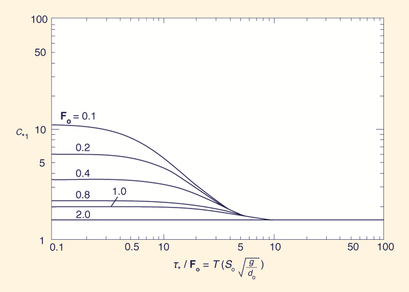
The next step in the analysis is to compare the propagation celerity c_*d and logarithmic decrement δ_d of the diffusion model with those of the full dynamic model. For F_o < 2, the propagation celerity of the diffusion wave, c_*d = 1.5, is a lower bound for the dynamic celerity. Since only the primary dynamic wave (that which travels downstream) is of interest here, the dynamic wave celerity will be referred to as c_*1.

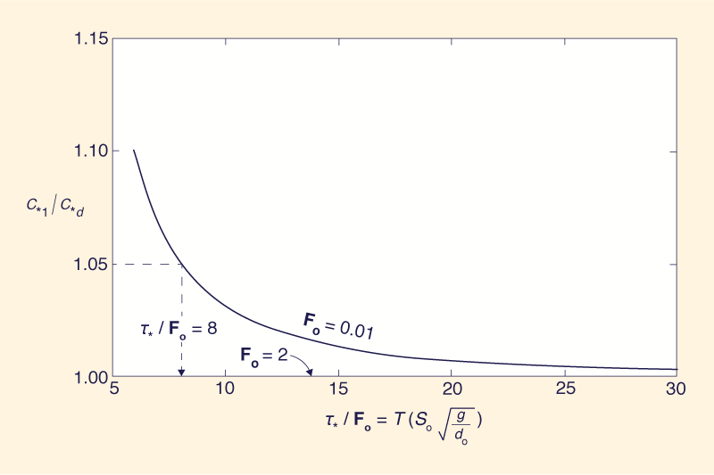
Figure 1 shows the variation of c_*1 as a function of τ_*/F_o. It can be seen from this figure that c_*1 tends to c_*d as τ_*/F_o increases, for all F_o. Figure 2 is an arithmetic plot of c_*1/c_*d versus τ_*/F_o for 5 ≤ τ_*/F_o ≤ 30. From this figure, for τ_*/F_o ≥ 8, the celerity error of the diffusion model is within 5%. The curve shown for F_o = 0.01 is an error bound.

Fig. 1.  Dimensionless celerity of dynamic model c*1 versus τ*/ Fo.

Fig. 2.  Ratio of celerities c*1/c*d versus τ*/Fo.

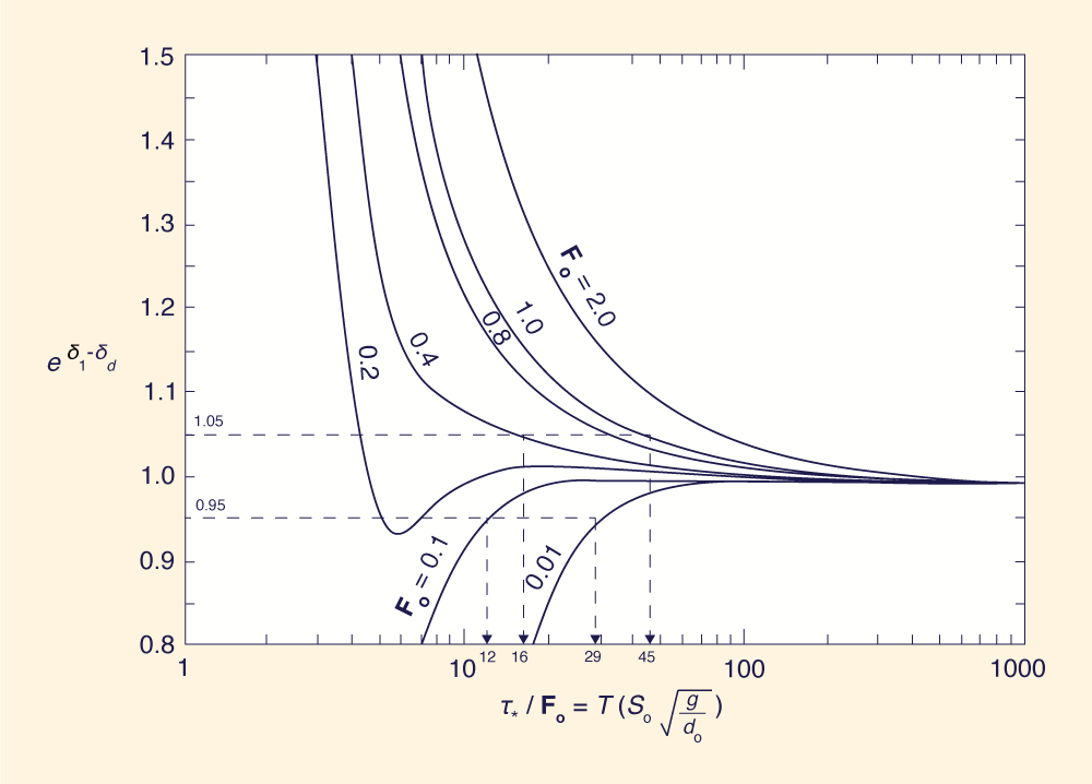
Keeping the celerity error to within 5% does not guarantee that the amplitude error will remain within the same tolerance. Figure 3 is a plot of e ^{δ₁ - δ_d} versus τ_*/F_o, in which δ₁ and δ_d are the logarithmic decrements of the dynamic and diffusion models, respectively. Figure 3 shows that for 0.1 ≤ F_o ≤ 0.4, τ_*/F_o > 16, for the attenuation error of the diffusion model to be within 5%. For a wider range of F_o, say, 0.01 ≤ F_o ≤ 1.0, τ_*/F_o ≥ 45. An exact value of the parameter τ_*/F_o for a given error defies generalization, being as it is a function of F_o. Nevertheless, from a practical standpoint, a value of τ_*/F_o > 30 is postulated (specific values of τ_*/F_o for a given F_o can be taken directly from Fig. 3).

Fig. 3.  Ratio of attenuation factors e δ1 - δd versus τ*/Fo.

Applying this criterion to the same example used before, for S_o = 0.0001 and d_o = 10 ft (3.05 m):

g        T So ( ____ ) 1/2  ≥ 30                 do

(17)

from which:

T ≥ 1.9 days

(18)

In the second example shown, for S_o = 0.01 and d_o = 1 ft (0.305 m):

T ≥ 8.8 min

(19)

On the basis of the examples shown, it is concluded that the diffusion model applies for a wider range of slopes and periods than the kinematic model, with the added advantage that the diffusion model does allow for physical attenuation. However, if inequality (Eq. 17) is not satisfied, the diffusion model breaks down and only the full dynamic model can properly account for the rate of travel and amount of attenuation of the wave.

---

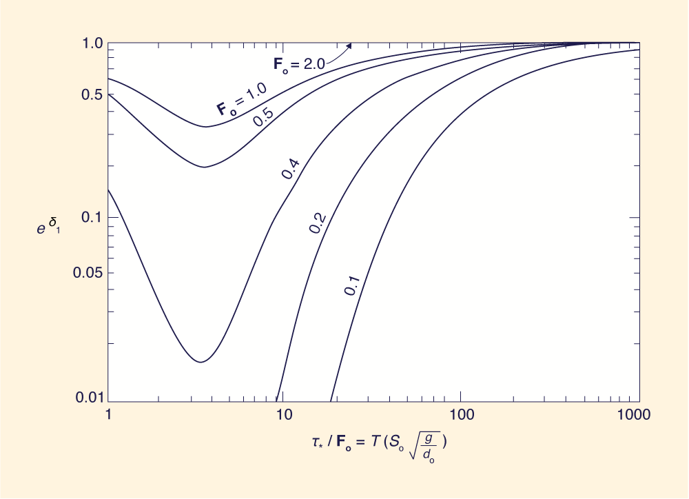
6.  FULL DYNAMIC MODEL

Figures 1 and 4 show c_*1 and e^δ₁ as a function of F_o and τ_*/F_o, respectively. For τ_*/F_o ≤ 30, i.e., the range where only the full dynamic model would apply, very strong attenuation is shown. For instance, for τ_*/F_o = 30, and F_o = 0.2, e^δ₁ = 0.23. This explains the nonpermanent characteristics of the dynamic wave: Once formed, it will attenuate quickly. In this regard, it is of interest to point out here the observations of Hayami (2) regarding the nonpermanent nature of dynamic disturbances in open channel flow. He reasoned that given all the irregularities present in natural river channels, it is striking that the general pattern of the flow closely resembles that of uniform (steady equilibrium) flow. The reason for this lies in the strong dissipative tendencies of dynamic disturbances, its nonpermanency being manifested in the appearance of uniform flow. Kinematic and diffusion waves, however, do not share the strong dissipative tendencies of dynamic waves due precisely to their long duration, or relatively large bed slopes, or both.

Fig. 4.  Attenuation factor of dynamic model e δ1 versus τ*/Fo.

---

7.  CONCLUSIONS

The applicability of the kinematic and diffusion models is assessed by comparing the propagation characteristics of sinusoidal perturbations to the steady uniform flow for the kinematic, diffusion, and dynamic models (the dynamic model is that based on the complete Saint Venant equations). The comparison allows the determination of inequality criteria that need to be satisfied if the kinematic or diffusion models are to simulate the physical phenomena within a prescribed accuracy.

It is shown that bed slope and wave period (akin to wave duration in waves of shape other than sinusoidal) are the important physical characteristics in determining the applicability of the approximate models. Larger bed slopes or long wave periods will satisfy the inequality criteria. In practice, larger bed slopes are those of overland flow, and long wave periods are those corresponding to slow-rising flood waves.

The diffusion model is shown to be applicable for a wider range of bed slopes and wave periods than the kinematic model. Where the two models break down, only the dynamic model will simulate the physical phenomena. The dynamic model, however, is shown to have markedly strong dissipative tendencies. This conclusion has had ample corroboration in the literature.

---

ACKNOWLEDGEMENTS

The writers wish to acknowledge the United States Environmental Protection Agency, Environmental Research Laboratory, Athens, Georgia, and the United States Department of Agriculture Forest Service, Rocky Mountain Forest and Range Experiment Station, Flagstaff, Arizona, for sponsoring this study.

---

APPENDIX I. EQUATIONS FOR PROPAGATION CELERITY c_* AND LOGARITHMIC DECREMENT δ

The equations for c_* and δ of the complete dynamic model are the following:

c*1 = 1 + D

(20a)

c*2 = 1 - D

(20b)

B  - E              δ1  = - 2 π   __________                        | 1 + D |

(21a)

B + E              δ2  = - 2 π   __________                         | 1 - D |

(21b)

in which A = (1/F_o²) - B ²;    B = 1/(σ_*F_o²);    C = (A ² + B ²)^1/2;    D = [(C + A)/ 2]^1/2; and E = [(C - A)/ 2]^1/2.

---

APPENDIX II. REFERENCES

Cunge, J. 1969. "On the Subject of a Flood Propagation Computation Method (Muskingum Method)," Journal of Hydraulic Research, Vol. 7, No. 2, 205-230. Hayami, S. 1951. "On the Propagation of Flood Waves," Bulletin of the Disaster Prevention Research Institute, Kyoto, Japan, Vol. 1, No. 1, Dec.. Lighthill, M. J., and G. B. Whitham, 1955. "On Kinematic Waves 1. Flood Movement in Long Rivers," Proceedings, Royal Society of London, London, England, Series A, Vol. 229, 281-316. Ponce, V. M., and D. B. Simons, 1977. "Shallow Wave Propagation in Open Channel Flow," Journal of the Hydraulics Division, ASCE, Vol. 103, HY12, Proc. Paper, 13392. Dec., 1461-1476. Wylie, C. R. 1966. Advanced Engineerings Mathematics, 3rd ed., McGraw-Hill Book Co. Inc., New York, N.Y.

---

APPENDIX III. NOTATION

    The following symbols are used in this paper:

α_o = wave amplitude at beginning of period;

α₁ = wave amplitude at end of period;

c = wave celerity. Eq. 1;

c_* = dimensionless wave celerity, Eq. 6;

d_o = steady uniform flow depth;

F_o = steady uniform flow Froude number;

g = acceleration of gravity;

L = wavelength;

L_o = reference channel length, Eq. 2;

S_o = bed slope;

u_o = steady uniform flow mean velocity;

T = wave period;

δ = logarithmic decrement, Eq. 7;

τ_* = dimensionless period, Eq. 5; and

σ_* = dimensionless wave number, Eq. 4.

---

Subscripts

1 = pertaining to primary dynamic wave (traveling downstream);

d = pertaining to diffusion model; and

k = pertaining to kinematic model.

---